
Variational Methods and 3D Tracking
Published:
This blog presents you with a lightweight real-time segmentation and pose tracking method which only uses only a monocular RGB camera and can run with multiple objects, and is robust to occlusion. You can watch the demonstration first to have a sense. The whole process is just mathematics which makes the output of each step predictable and allows us to have insight for further improvement. Real-Time Monocular Segmentation and Pose Tracking.
Preliminaries
Let $I$ be the image in the image domain $\Omega \subset \mathbb{R}^2$. With every pixel $\textbf{x} = [x, y]^T$, there is a corresponding color $\textbf{c} = I(x, y)$ (this can be grey value or RGB).
The 3D model will be transformed from its model space into camera space by a transformation matrix $T$ (our camera is fixed at the origin and looks in the positive direction of $z$ axis - a little bit different from OpenGL). The rigid transformation matrix $T$ we call pose of 3D model and is presented by a $4 \times 4$ homogeneous matrix:
\[T = \left[\begin{matrix} R & \textbf{t} \\ \textbf{0} & 1 \\ \end{matrix}\right] \in \mathbb{SE}(3)\]with $R \in \mathbb{SO}(3)$ and $\textbf{t} \in \mathbb{R}^3$.
To understand more about the definition of $\mathbb{SE}(3)$ (Lie-group Special Euclidean) as well as its properties, we recommend you to read chapter 2 of the book: An Invitation to 3-D Vision.
Another assumption of this tracking problem is that we must have the intrinsic matrix $K$ of our camera. This can be achieved easily by estimating the matrix with multiple checkerboard images captured beforehand.
\[K = \left[ \begin{matrix} f_x & 0 & c_x \\ 0 & f_y & c_y \\ 0 & 0 & 1 \end{matrix} \right]\]With a point in a 3D model $\textbf{X}_i = [X_i, Y_i, Z_i, 1]^T$ (represented in homogeneous coordinate), its project in 2D image is:
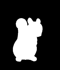
\[Z'\textbf{x} = Z'\left[\begin{matrix} x \\ y \\ 1 \end{matrix}\right] = \left[\begin{matrix} f_x & 0 & c_x \\ 0 & f_y & c_y \\ 0 & 0 & 1 \end{matrix}\right] \left[\begin{matrix} 1 & 0 & 0 & 0 \\ 0 & 1 & 0 & 0 \\ 0 & 0 & 1 & 0 \end{matrix}\right] \left[\begin{matrix} r_{11} & r_{12} & r_{13} & t_1 \\ r_{21} & r_{22} & r_{23} & t_2 \\ r_{31} & r_{32} & r_{33} & t_3 \\ 0 & 0 & 0 & 1 \end{matrix}\right] \left[\begin{matrix} X_i \\ Y_i \\ Z_i \\ 1 \end{matrix}\right]\]The silhouette of a 3D model in an image plane after projection splits the image into two regions: foreground $\Omega_f \subset \Omega$ and background $\Omega_b = \Omega \setminus \Omega_f$. In the figure below, the white region is the foreground, and the rest (black color) is the background.
For pose tracking, the goal of the problem is to find the pose of the 3D model in each frame. With an assumption that the pose $T_k$ of frame $I_k$ is already known, we only need to perform pose tracking at frame $I_{k+1}$. Because of the linearity of transformation, the pose of the next frame can be expressed by the current pose according to this equation: $T_{k+1} = \Delta T T_{k}$. So, for each new frame, we just need to find $\Delta T$ to rectify the current pose $T_k$.
For pose optimization, we model the rigid body motion $\Delta T$ with twists:
\[\hat{\xi} = \left[ \begin{matrix} \hat{\textbf{w}} & \textbf{v} \\ \textbf{0} & 0 \\ \end{matrix}\right] \in \mathfrak{se}(3)\]with $\textbf{w} \in \mathfrak{so}(3)$ and $\textbf{v} \in \mathbb{R}^3$.
Each twist is parametrized by a six-dimensional vector of so-called twist coordinates:
\[\xi = [\omega_1, \omega_2, \omega_3, v_1, v_2, v_3]^T \in \mathbb{R}^6\]and the matrix exponential:
\[\Delta T = \operatorname{exp}(\hat{\xi}) \in \mathbb{SE}(3)\]Statistical Image Segmentation
Shape Kernel $\Phi$
The approach of this method is mainly based on statistical segmentation (you can read our blog here), so as usual the silhouette of the 3D model will be implicitly represented by a so-called shape kernel $\Phi$. This is called the level-set embedding function, and the $\Phi$ must have the properties:
\[\begin{equation*} \begin{cases} C &= \{(x, y) \in \Omega \, | \, \phi(x, y) = 0\} \\ \operatorname{inside} (C) &= \{(x, y) \in \Omega \, | \, \phi(x, y) \lt 0\} \\ \operatorname{outside} (C) &= \{(x, y) \in \Omega \, | \, \phi(x, y) \gt 0\} \end{cases} \end{equation*}\]where $C$ is the contour of the silhouette (image below).
| Silhouette | Contour |
|---|---|
| 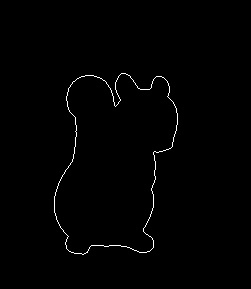 |
To present $\Phi$, we use a signed distance function:
\[d(\textbf{x}) = \underset{\textbf{x}_c \in C}{\operatorname{min}}|\textbf{x} - \textbf{x}_c|\] \[\begin{equation*} \Phi(\textbf{x}) = \begin{cases} -d(\textbf{x}) \quad \forall \textbf{x} \in R_f \\ d(\textbf{x}) \quad \forall \textbf{x} \in R_b \end{cases} \end{equation*}\]where $R_f$ is foreground region and $R_b$ is background region.
| Signed Distance Function | Heatmap |
|---|---|
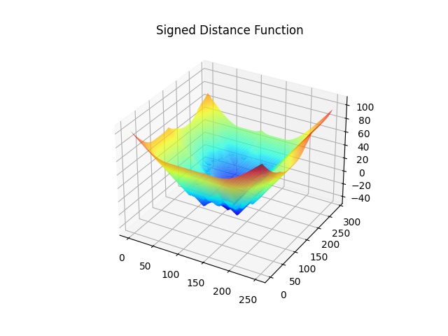 | 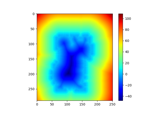 |
To calculate the signed distance function efficiently, you can read [6]
Generative Model
It is extremely challenging if there is no assumption for an inverse problem like this. To reduce the complexity of the problem, Victor et al. [1] proposed a graphical model. Let’s have a look at it:
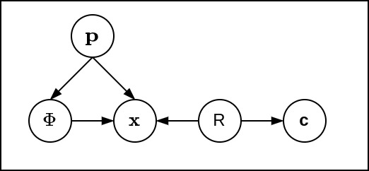
where
- $\textbf{p}$: pose of 3D object (6 DoF) parameterized by a twist coordinate $\xi$.
- $\Phi$: is the shape kernel (as defined before).
- $\textbf{x}$: is 2D coordinate of a pixel in image plane - $\textbf{x} = (x, y) \in \Omega \subset \mathbb{R}^2$.
- $R$: is random region variable $R$, can be foreground or background - $R \in {R_f, R_b}$.
- $\textbf{c}$: is RGB color - $\textbf{c} \in [0, 255] \times[0, 255] \times [0, 255]$
This graphical model makes sense since the random variable pose of the 3D model will affect the shape kernel $\Phi$ through its silhouette. The probability random variable $\textbf{x}$ in the image plane would depend on pose $\textbf{p}$, the region $R$ whether foreground or background and $\Phi$. And finally, the probability of color $\textbf{c}$ definitely depends on the region $R$.
Our goal now is to maximize a posteriori $P(\Phi, \textbf{p} \mid \Omega)$ with give image $I \subset \Omega$. However, first, let’s have a look at generative model $P(\textbf{x}, \textbf{c}, R, \Phi, \textbf{p})$:
\[P(\textbf{x}, \textbf{c}, R, \Phi, \textbf{p}) = P(\textbf{x} \mid R, \Phi, \textbf{p}) \, P(\textbf{c} \mid R) \, P(R) \, P(\Phi \mid \textbf{p}) \, P(\textbf{p})\]Expand it by dividing both sides by: \(P(\textbf{c}) = \sum_{R \in {R_f, R_b}} P(\textbf{c} \mid R) \, P(R)\)
to get:
\[P(\textbf{x}, R, \Phi, \textbf{p} \mid \textbf{c}) = P(\textbf{x} \mid R, \Phi, \textbf{p}) \, P(R \mid \textbf{c}) \, P(\Phi \mid \textbf{p}) \, P(\textbf{p})\]where: \(P(R_j \mid \textbf{c}) = \dfrac{P(\textbf{c} | R_j) \, P(R_j)}{\sum_{i = \{f, b\}} P(\textbf{c} | R_i) \, P(R_i)} \qquad j = \{f, b\}\)
Next, marginalize over $R$:
\[P(\textbf{x}, \Phi, \textbf{p} \mid \textbf{c}) = \sum_{i=\{f, b\}} P(\textbf{x} \mid R_i, \Phi, \textbf{p}) \, P(R_i \mid \textbf{c}) \, P(\Phi \mid \textbf{p}) \, P(\textbf{p})\]And divide by $P(\textbf{x})$:
\[P(\Phi, \textbf{p} \mid \textbf{c}, \textbf{x}) = \dfrac{1}{P(\textbf{x})}\sum_{i=\{f, b\}} P(\textbf{x} \mid R_i, \Phi, \textbf{p})\, P(R_i \mid \textbf{c}) \, P(\Phi \mid \textbf{p}) \, P(\textbf{p})\]Since we can assume that $P(\textbf{x})$ is a constant (for the sake of simplicity), the posterior of a given pixel and its color can be written as:
\[P(\Phi, \textbf{p} \mid \textbf{c}, \textbf{x}) \propto \sum_{i=\{f, b\}} P(\textbf{x} \mid R_i, \Phi, \textbf{p})\, P(R_i \mid \textbf{c}) \, P(\Phi \mid \textbf{p}) \, P(\textbf{p})\]And final posterior over an image is:
\[P(\Phi, \textbf{p} \mid \Omega) \propto \prod_{\textbf{x, c} \in \Omega } \sum_{i=\{f, b\}} \{P(\textbf{x} \mid R_i, \Phi, \textbf{p})\, P(R_i \mid \textbf{c})\} \, P(\Phi \mid \textbf{p}) \, P(\textbf{p})\]To reduce the complexity, Victor et al. [1] eliminated the prior term to get a simple version which makes maximizing a posterior become maximizing likelihood.
\[P(\Phi, \textbf{p} \mid \Omega) \propto \prod_{\textbf{x, c} \in \Omega } \sum_{i=\{f, b\}} \{P(\textbf{x} \mid R_i, \Phi, \textbf{p})\, P(R_i \mid \textbf{c})\}\]Maximizing likelihood is also equivalent to minimizing negative logarithm likelihood:
\[\underset{\textbf{p}}{\operatorname{arg min}} \log{P(\Phi, \textbf{p}\mid \Omega)} = \sum_{\textbf{x}, \textbf{c}\in \Omega} -\operatorname{log}\left(\sum_{i=\{f, b\}} P(\textbf{x} \mid R_i, \Phi, \textbf{p})\, P(R_i \mid \textbf{c})\right)\]Minimize Negative Logarithm Likelihood
Our goal now is to minimize the negative logarithm likelihood:
\[\underset{\textbf{p}}{\operatorname{arg min}} \log{P(\Phi, \textbf{p}\mid \Omega)} = \sum_{\textbf{x}, \textbf{c}\in \Omega} -\operatorname{log}\left(\sum_{i=\{f, b\}} P(\textbf{x} \mid R_i, \Phi, \textbf{p})\, P(R_i \mid \textbf{c})\right)\]To solve this optimization problem, we need to know the explicit probability of each term in the equation:
- Let start first with pixel likelihood $P(\textbf{x} \mid R_f, \Phi, \textbf{p})$.
![]()
Intuitively, the likelihood probability of a red pixel in foreground $R_f$ and background $R_b$ will be:
\[\begin{aligned} P(\textbf{x} \mid R_f, \Phi, \textbf{p}) &= \dfrac{1}{\operatorname{Area}_f} \\ P(\textbf{x} \mid R_b, \Phi, \textbf{p}) &= 0 \end{aligned}\]and that of the green pixel in foreground $R_f$ and background $R_b$ will be:
\[\begin{aligned} P(\textbf{x} \mid R_f, \Phi, \textbf{p}) &= 0 P(\textbf{x} \mid R_b, \Phi, \textbf{p}) &= \dfrac{1}{\operatorname{Area}_b} \end{aligned}\]To generalize both expressions, we can utilize the shape kernel property.
We already know:
\[\begin{equation*} \begin{cases} C &= \{(x, y) \in \Omega \, | \, \phi(x, y) = 0\} \\ \operatorname{inside} (C) &= \{(x, y) \in \Omega \, | \, \phi(x, y) \lt 0\} \\ \operatorname{outside} (C) &= \{(x, y) \in \Omega \, | \, \phi(x, y) \gt 0\} \end{cases} \end{equation*}\]So, with the introduction of a Heaviside function:
\[\begin{equation*} H(x) = \begin{cases} 1 & \quad x \le 0, \\ 0 & \quad x \gt 0. \end{cases} \end{equation*}\]the above two probabilities can be written as:
\[\begin{aligned} P(\textbf{x} \mid R_f, \Phi, \textbf{p}) &= \dfrac{H(\Phi(\textbf{x}))}{\eta_f} \\ P(\textbf{x} \mid R_b, \Phi, \textbf{p}) &= \dfrac{1 - H(\Phi(\textbf{x}))}{\eta_b} \end{aligned}\]where
\[\begin{aligned} \eta_f &= \sum_{i = 1}^{N}H(\Phi(\textbf{x})) \\ \eta_b &= \sum_{i = 1}^{N}1 - H(\Phi(\textbf{x})) \end{aligned}\]- Second is region posterior $P(R_i \mid \textbf{c})$.
Based on Bayes’ rule, we can get:
\[P(R_f \mid \textbf{c}) = \dfrac{P(\textbf{c} \mid R_f) P(R_f)}{P(\textbf{c} \mid R_f) P(R_f) + P(\textbf{c} \mid R_b) P(R_b)}\] \[P(R_b \mid \textbf{c}) = \dfrac{P(\textbf{c} \mid R_b) P(R_b)}{P(\textbf{c} \mid R_f) P(R_f) + P(\textbf{c} \mid R_b) P(R_b)}\]where:
\[\begin{aligned} P(R_f) &= \dfrac{\eta_f}{\eta} \\ P(R_b) &= \dfrac{\eta_b}{\eta} \\ \eta &= \eta_f + \eta_b \end{aligned}\]Two likelihood $P(\textbf{c} \mid R_f)$ and $P(\textbf{c} \mid R_b)$ are simply represented by two $32\times32\times32$ - bin histograms.
\[\begin{aligned} E(\Phi, \textbf{p}) &= \sum_{\textbf{x}, \textbf{c} \in \Omega} -\operatorname{log}(\dfrac{H(\Phi(\textbf{x}))}{\eta_f}\dfrac{P(\textbf{c} \mid R_f)\eta_f}{P(\textbf{c} \mid R_f) \eta_f+ P(\textbf{c} \mid R_b) \eta_b} \\ &+ \dfrac{1 - H(\Phi(\textbf{x}))}{\eta_b}\dfrac{P(\textbf{c} \mid R_b)\eta_b}{P(\textbf{c} \mid R_f) \eta_f+ P(\textbf{c} \mid R_b) \eta_b} )\\ &= \sum_{\textbf{x}, \textbf{c} \in \Omega} -\operatorname{log} \left(H(\Phi(\textbf{x})) P_f + (1 - H(\Phi(\textbf{x})))P_b\right) \end{aligned}\]where:
\[P_f = \dfrac{P(\textbf{c} \mid R_f)}{P(\textbf{c} \mid R_f) \eta_f+ P(\textbf{c} \mid R_b) \eta_b}\] \[P_b = \dfrac{P(\textbf{c} \mid R_b)}{P(\textbf{c} \mid R_f) \eta_f+ P(\textbf{c} \mid R_b) \eta_b}\]Finally, we have the objective function for the optimization problem:
\[\begin{aligned} E(\textbf{p}) &= \sum_{\textbf{x}, \textbf{c} \in \Omega} -\operatorname{log} (H(\Phi(\textbf{x})) P_f + (1 - H(\Phi(\textbf{x})))P_b) \\ &= \sum_{\textbf{x}, \textbf{c} \in \Omega} F(\textbf{x}, \textbf{c}) \end{aligned}\]Optimize Energy Function
For the rest of the blog, we will use $\xi$ instead of pose $\textbf{p}$.
To find $\xi$ such that energy function $E(\xi)$ is minimum, the numerical optimization method Gauss - Newton is chosen because of its fast convergence. However, the energy function is not in linear form, so we need to rewrite it before applying Gauss - Newton strategy:
\[E(\xi) = \dfrac{1}{2}\sum_{\textbf{x}, \textbf{c} \in \Omega} \dfrac{1}{\psi(\textbf{x}, \textbf{c})}F^2(\textbf{x}, \textbf{c})\]where:
\[\psi(\textbf{x}, \textbf{c}) = F(\textbf{x}, \textbf{c})\]is considered a constant when optimizing.
Gauss - Newton Strategy
The Jacobian and pseudo-Hessian matrix are:
\[\begin{aligned} \dfrac{\partial E(\xi)}{\partial\xi} &= \dfrac{1}{2}\sum_{\textbf{x}, \textbf{c} \in \Omega}\psi(\textbf{x}, \textbf{c})\dfrac{\partial F^2(\textbf{x}, \textbf{c})}{\partial \xi} = \sum_{\textbf{x}, \textbf{c} \in \Omega}\psi(\textbf{x}, \textbf{c})F\dfrac{\partial F}{\partial \xi} \\ \dfrac{\partial^2 E(\xi)}{\partial\xi^2} &= \sum_{\textbf{x}, \textbf{c} \in \Omega}\psi(\textbf{x}, \textbf{c})\left( \left(\dfrac{\partial F}{\partial \xi}\right)^T\dfrac{\partial F}{\partial \xi} + F\dfrac{\partial^2 F}{\partial \xi^2} \right) \end{aligned}\]Approximating the energy function with Taylor series and the Hessian matrix by pseudo-Hessian:
\[E(\xi + \Delta\xi) \approx E(\xi) + \sum_{\Omega}J\Delta\xi + \dfrac{1}{2}\sum_{\Omega}\psi(\textbf{x})\Delta\xi^TJ^TJ\Delta\xi\]When we reach optimum, this $E(\xi + \Delta\xi) \approx E(\xi)$ should happen which makes:
\[\begin{aligned} \sum_{\Omega}J\Delta\xi + \dfrac{1}{2}\sum_{\Omega}\psi(\textbf{x})\Delta\xi^TJ^TJ\Delta\xi &= 0 \\ \Rightarrow \left(\sum_{\Omega}J + \dfrac{1}{2}\sum_{\Omega}\psi(\textbf{x})\Delta\xi^TJ^TJ\right)\Delta\xi &= 0 \\ \end{aligned}\]Since $\Delta \xi$ can not be zero, so:
\[\sum_{\Omega}J + \dfrac{1}{2}\sum_{\Omega}\psi(\textbf{x})\Delta\xi^TJ^TJ = 0\]which leads:
\[\Delta\xi = -\left(\sum_\Omega\psi(x)J^TJ\right)^{-1}\left(\sum_\Omega J\right)\]The current pose is updated with:
\[T \leftarrow \operatorname{exp}(\Delta \hat{\xi})T\]Chain rule
We already have an updated equation for $\Delta \xi$; what remains is how we construct the Jacobian and pseudo-Hessian matrix.
\[F(\textbf{x}, \textbf{c}) = -\operatorname{log} (H(\Phi(\textbf{x})) P_f + (1 - H(\Phi(\textbf{x})))P_b)\]This is pretty easy, thanks to the chain rule:
\[J = \dfrac{P_b - P_f}{H(\Phi(\textbf{x})) P_f + (1 - H(\Phi(\textbf{x})))P_b} \delta(\Phi(x)) \dfrac{\partial \Phi(\textbf{x})}{\partial \xi}\]where Dirac function $\delta(.)$ is derivative of Heaviside function $H(.)$. In the implementation, the smooth Heaviside is used.
\[H(x) = \dfrac{1}{\pi} \left(-\operatorname{atan}(\epsilon \cdot x) + \dfrac{\pi}{2}\right)\]with $\epsilon = 0.1$.
Next is derivative of $\dfrac{\partial \Phi(\textbf{x})}{\partial \textbf{p}}$.
Based on the chain rule, we have:
\[\dfrac{\partial \Phi(\textbf{x})}{\partial \xi} = \dfrac{\partial \Phi}{\partial \textbf{x}} \dfrac{\partial \textbf{x}}{\partial \xi}\]The first term $\dfrac{\partial \Phi}{\partial \textbf{x}}$ is approximated by central difference:
\[\left[\dfrac{\partial \Phi(\textbf{x})}{\partial x}, \dfrac{\partial \Phi(\textbf{x})}{\partial y}\right] = \left[ \begin{matrix} \Phi_y \\ \Phi_x \end{matrix} \right]^T = \left[ \begin{matrix} \dfrac{\Phi(x + 1, y) - \Phi(x - 1, y)}{2} \\ \dfrac{\Phi(x, y + 1) - \Phi(x, y - 1)}{2} \end{matrix} \right]^T\]While the second term $\dfrac{\partial \textbf{x}}{\partial \xi}$ is:
To remind you of the projection equation, we write the equation again here with a little change:
\[Z\textbf{x} = Z\left[\begin{array}{c} x \\ y \\ 1 \end{array}\right] = \left[\begin{array}{ccc} f_x & 0 & c_x \\ 0 & f_y & c_y \\ 0 & 0 & 1 \end{array}\right] \left[\begin{array}{cccc} 1 & 0 & 0 & 0 \\ 0 & 1 & 0 & 0 \\ 0 & 0 & 1 & 0 \end{array}\right] \operatorname{exp}(\hat{\xi}) \left[\begin{array}{c} X' \\ Y' \\ Z' \\ 1 \end{array}\right]\]where $[X’, Y’, Z’, 1]^T$ is the current position of a point $[X, Y, Z, 1]^T$ at the current frame.
We assume that the movement of the object between 2 frames is really small, the approximation below is true:
\[\operatorname{exp}(\hat{\xi}) = \mathbb{I}_{4\times4} + \hat{\xi}\]The second term $\dfrac{\partial \textbf{x}}{\partial \xi}$ is:
\[\dfrac{\partial \textbf{x}}{\partial \xi} = \left[ \begin{array}{ccc} \dfrac{f_x}{Z'} & 0 & -\dfrac{X'f_x}{(Z')^2} \\ 0 & \dfrac{f_y}{Z'} & -\dfrac{Y'f_y}{(Z')^2} \end{array} \right] \left[ \begin{array}{cccccc} 0 & Z' & -Y' & 1 & 0 & 0 \\ -Z' & 0 & X' & 0 & 1 & 0 \\ Y' & -X' & 0 & 0 & 0 & 1 \\ \end{array} \right]\]Some of you may ask how we can know the depth value $Z’$.
Obviously, because we project the 3D model into the image plane, we definitely can know this (we are kings in computer graphics). In OpenGL, we can access depth map by the function glReadPixel, but with openGLES, a little trick is required that we have to compact depth values in fragment shader into RGBA value and render it before accessing with glReadPixel since openGLES doesn’t support reading depth map operator, but there will be small errors.
Rendering
Because our camera is a little bit different from the normal schema in OpenGL that is, our camera simulates the real camera looking in the positive direction of $z$ axis. So, the look-at matrix and projection matrix would be different.
\[\begin{aligned} L &= \left[ \begin{matrix} 1 & 0 & 0 & 0 \\ 0 & -1 & 0 & 0 \\ 0 & 0 & -1 & 0 \\ 0 & 0 & 0 & 1 \end{matrix} \right] \\ P &= \left[ \begin{matrix} \dfrac{2f_x}{w} & 0 & 1 - \dfrac{2c_x}{w} & 0 \\ 0 & -\dfrac{2f_y}{h} & \dfrac{2c_y}{h} -1 & 0 \\ 0 & 0 & -\dfrac{Z_f + Z_n}{Z_f - Z_n} & -\dfrac{2Z_fZn}{Z_f - Z_n} \\ 0 & 0 & -1 & 0 \end{matrix} \right] \\ \end{aligned}\]To know how to construct the matrices, visit this.
Demonstration
<iframe width="560" height="315" src="https://www.youtube.com/embed/V0rqnS49Jmo" title="YouTube video player" frameborder="0" allow="accelerometer; autoplay; clipboard-write; encrypted-media; gyroscope; picture-in-picture" allowfullscreen></iframe>
<iframe width="560" height="315" src="https://www.youtube.com/embed/zMS4lG3k6I8" title="YouTube video player" frameborder="0" allow="accelerometer; autoplay; clipboard-write; encrypted-media; gyroscope; picture-in-picture" allowfullscreen></iframe>
Reference
To comprehend the whole system, we recommend you read [1], [2], [3], [4] and [5] for further improvement in speed.
[1] Prisacariu, Victor A., and Ian D. Reid. “PWP3D: Real-time segmentation and tracking of 3D objects.” International journal of computer vision 98.3 (2012): 335-354.
[2] Prisacariu, Victor Adrian, et al. “Real-time 3d tracking and reconstruction on mobile phones.” IEEE transactions on visualization and computer graphics 21.5 (2014): 557-570.
[3] Bibby, Charles, and Ian Reid. “Robust real-time visual tracking using pixel-wise posteriors.” European conference on computer vision. Springer, Berlin, Heidelberg, 2008.
[4] Tjaden, Henning, et al. “A region-based gauss-newton approach to real-time monocular multiple object tracking.” IEEE transactions on pattern analysis and machine intelligence 41.8 (2018): 1797-1812.
[5] Stoiber, Manuel, et al. “A sparse gaussian approach to region-based 6DoF object tracking.” Proceedings of the Asian Conference on Computer Vision. 2020.
[6] Felzenszwalb, Pedro F., and Daniel P. Huttenlocher. “Distance transforms of sampled functions.” Theory of computing 8.1 (2012): 415-428.