
Variational Methods and 3D Reconstruction
Published:
There are numerous methods for reconstructing a real object into the mesh, such as voxel carving, which independently processes the input images or structure from motion. However, in this blog, we would like to introduce to you another solution for this ill-posed inverse computer vision problem. This method is a volumetric approach, where each voxel is assigned two probability values for being in or out of the 3D object. Let’s start.
Probabilistic Multiple - View 3D Reconstruction
Preliminaries
Before diving into the main sections, we have to go through notations first.
Volume
Let volume $V$ be our local 3D environment, which includes the 3D object needed to reconstruct.
\[V := [v_{11}, v_{12}] \times [v_{21}, v_{22}] \times [v_{31}, v_{32}] \subset \mathbb{R}^3\]and each $v_{ij} \in \mathbb{R}$.
where:
$[a, b] = { x \mid a \le x \le b }$
$A \times B = {(a, b) \mid a \in A \, \text{and} \, b \in B }$ is Cartesian product of two sets.
Example:
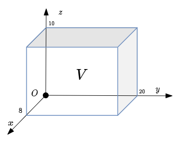
In $x$ axis, the volume $V$ in the image above goes from $0$ to $8$, from $0$ to $20$ for $y$ axis and from $0$ to $10$ for $z$ axis.
Discretely, volume $V$ having a resolution $N_x \times N_y \times N_z$ is a set of voxels:
\[V :=\left\{\left(\begin{matrix} v_{11} + i \cdot \dfrac{v_{12} - v_{11}}{N_x} \\ v_{21} + j \cdot \dfrac{v_{22} - v_{21}}{N_y} \\ v_{31} + k \cdot \dfrac{v_{32} - v_{31}}{N_x} \\ \end{matrix}\right) \Bigg\vert \quad \begin{matrix} i = 0,..., N_x - 1 \\ j = 0,..., N_y - 1 \\ k = 0,..., N_z - 1 \\ \end{matrix}\right\}\]Images and Projection
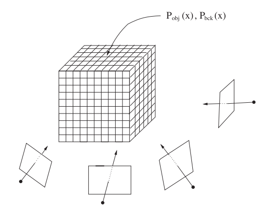
Let the sequence of input RGB images be:
\[I_1, ..., I_n: \Omega \mapsto \mathbb{R}^3\]and the known model view projection matrices corresponding to input RGB images respectively be:
\[\pi_1, ..., \pi_n : V \mapsto \Omega\]where $\Omega \subset \mathbb{R}^2$.
Shape Function
We present the 3D object by a function $u$. The definition of $u$ is:
\[u(\textbf{v}) = \begin{cases} 1 \qquad \textbf{v} \in \text{3D object} \\ 0 \qquad \text{otherwise} \end{cases}\]where $\textbf{v}$ is a 3D coordinate of a voxel in volume $V$.
In summary, the inputs of our 3D reconstruction problem include:
- Sequence of images ${I_i}$
- Sequence of model - view - projection matrices ${\pi_i}$ corresponding
What we need to find is so-called shape function $u(.)$.
Generative Model
It is extremely challenging if there is no assumption for an inverse problem like this. To reduce the complexity of the problem, Victor et al. [1] proposed a graphical model. Let’s have a look at it:
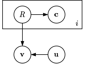
where:
- $i$: the index of a frame - $i = 1…n$.
- $R$: is a random region variable, can be foreground or background - $R \in {R_f, R_b}$
- $\textbf{c}$: color of voxel after being projected to $i^{th}$ image - $\textbf{c} \in \mathbb{R}^3$
- $\textbf{v}$: voxel coordinate in volume $V$ - $\textbf{v} \in \mathbb{R}^3$
- $\textbf{u}$: $= u(\textbf{v})$
This graphical model may be biased to the heuristic of designers, but at some point, it is still valid. The random variable $\textbf{v}$ in $V$ depends on not only the shape of the 3D object (obviously) but also the foreground or background region $R$ that its projection to image planes belongs to. Whereas the variable color $\textbf{c}$ undoubtedly depends on the region $R$.
Maximizing A Posteriori
Our goal is to find shape function $\textbf{u}$ given ${ I_i, \pi_i}$ or in statistical perspective, we need to seek $\textbf{u}$ such that posteriori $P(\textbf{u} \mid \textbf{v}, \textbf{c}_{1…n})$ is maximum.
To derive formulation for this posterior, first let’s start with the joint distribution for a given voxel $P(\textbf{u}, \textbf{v}, R_{1…n}, \textbf{c}_{1…n})$:
\[P(\textbf{u}, \textbf{v}, R_{1...n}, \textbf{c}_{1...n}) = P(\textbf{v} \mid \textbf{u}, \textbf{v}, R_{1...n}) P(\textbf{c}_{1...n} \mid R_{1...n}) P(R_{1...n}) P(\textbf{u})\]We divide both sides by \(P(\textbf{c}_{1...n}) = \underset{i \in {\{f, b\}}}{\sum}P(\textbf{c}_{1...n} \mid R_{i, 1...n}) P(R_{i, 1...n})\) to get:
\[P(\textbf{u}, \textbf{v}, R_{1...n} \mid \textbf{c}_{1...n}) = P(\textbf{v} \mid \textbf{u}, \textbf{v}, R_{1...n}) P(R_{1...n} \mid \textbf{c}_{1...n}) P(\textbf{u})\]Next, we marginalize over $P(R_{1…n})$:
\[P(\textbf{u}, \textbf{v} \mid \textbf{c}_{1...n}) = \underset{i \in \{ j, b\}}{\sum} P(\textbf{v} \mid \textbf{u}, \textbf{v}, R_{i, 1...n}) P(R_{i, 1...n} \mid \textbf{c}_{1...n}) P(\textbf{u})\]With assumption that $P(\textbf{v})$ is constant, we can omit the random variable $\textbf{v}$ by divide $P(\textbf{u}, \textbf{v} \mid \textbf{c}_{1…n})$ by $P(\textbf{v})$:
\[P(\textbf{u} \mid \textbf{v}, \textbf{c}_{1...n}) \propto \underset{i \in \{ j, b\}}{\sum} P(\textbf{v} \mid \textbf{u}, \textbf{v}, R_{i, 1...n}) P(R_{i, 1...n} \mid \textbf{c}_{1...n}) P(\textbf{u})\]The prior $P(\textbf{u})$ is also eliminated for the sake of simplicity. Finally, the posterior over the volume becomes likelihood:
\[\begin{aligned} P(u \mid \Omega_3) &\propto \underset{\textbf{v} \in \Omega_3}{\prod} P(\textbf{u} \mid \textbf{v}, \textbf{c}_{1...n}) \\ &\propto \underset{\textbf{v} \in \Omega_3}{\prod}\left\{\sum_{i\in \{ f, b\}} P(\textbf{v} \mid \textbf{u}, \textbf{v}, R_{i, 1...n}) P(R_{i, 1...n} \mid \textbf{c}_{1...n})\right\} \end{aligned}\]The posterior has revealed its formulation, but we still have not known each small term in it.
- For the region posterior, we can get its equation by applying Bayes’ rule:
- Regarding voxel likelihood, intuitively, we have:

For a red voxel inside our 3D object (cylinder in the example), its probability would be:
\[\begin{aligned} P(\textbf{v} \mid \textbf{u}, R_{f, 1...n}) &= \dfrac{1}{\text{volume}_f} \\ P(\textbf{v} \mid \textbf{u}, R_{b, 1...n}) &= 0 \end{aligned}\]For a gree voxel outside our 3D object (cylinder in the example), its probability would be:
\[\begin{aligned} P(\textbf{v} \mid \textbf{u}, R_{f, 1...n}) &= 0 \\ P(\textbf{v} \mid \textbf{u}, R_{b, 1...n}) &= \dfrac{1}{\text{volume}_b} \end{aligned}\]Without loss of generality, with shape function $\textbf{u}$, we can have a general formulation of a voxel likelihood:
\[\begin{aligned} P(\textbf{v} \mid \textbf{u}, R_{f, 1...n}) &= \dfrac{\textbf{u}}{\zeta_f} \\ P(\textbf{v} \mid \textbf{u}, R_{b, 1...n}) &= \dfrac{1 - \textbf{u}}{\zeta_b} \end{aligned}\]and $\zeta_f, \zeta_b$ being the average number of voxels (over n views) that project to a foreground pixel (with $P(\textbf{c} \mid R_f) \gt P(\textbf{c} \mid R_b)$ and $\textbf{c} = I_m(\pi_m(\textbf{v}))$) and a background pixel, respectively.
Now, one question has come is that how can we compute two probabilities \(P(\textbf{c}_{1...n} \mid \textbf{R}_{i,1...n})\) with \(i \in \{ f, b\}\). A straightforward way is to treat \(\{P(\textbf{c}_k \mid R_{i, k})\}\) independently. Based on visibility, the probability of a voxel in the foreground is equivalent to the probability that all cameras observe this voxel in the foreground, whereas the probability of a voxel being a part of the background is that at least one camera sees it as the background. This way is pretty similar to voxel carving when a voxel is considered as background if its projections on the background.
\[\begin{aligned} P(\textbf{c}_{1...n} \mid R_{f, 1...n}) &= \prod_{k=1}^nP(\textbf{c}_k \mid R_{f, k}) \\ P(\textbf{c}_{1...n} \mid R_{b, 1...n}) &= 1 - \prod_{k=1}^n\{1 - P(\textbf{c}_k \mid R_{b, k}) \} \end{aligned}\]We can describe \(P(\textbf{c}_k \mid R_{i, k})\) by Gaussian distribution or simply with a histogram.
However, these joint probabilities are not calculated easily since their products tend to be very small. To overcome this, they are rewritten:
\[\begin{aligned} P(\textbf{c}_{1...n} \mid R_{f, 1...n}) &= \operatorname{exp} \left( \dfrac{\sum_{k = 1}^n\operatorname{log}P(\textbf{c}_k \mid R_{f, k})}{n} \right) \\ P(\textbf{c}_{1...n} \mid R_{b, 1...n}) &= 1 - \operatorname{exp} \left( \dfrac{\sum_{k = 1}^n1 - \operatorname{log}( 1 - P(\textbf{c}_k \mid R_{b, k}))}{n} \right) \end{aligned}\]The probability of foreground and background region over $n$ views becomes $P(R_{f, 1…n}) = \dfrac{\bar{\eta_f}}{\eta}$ with $\eta_f$ being the average value of foreground area $\eta_f$ over the $n$ views. $P(R_{b, 1…n})$ follows analogously ($\eta$ is the whole image area).
So the final posterior equation is:
\[E = P(u \mid \Omega_3) = \prod_{\textbf{v} \in \Omega_3}\{ \textbf{u}P_i + (1 - \textbf{u})P_o\}\]where:
\[\begin{aligned} P_i &= \dfrac{\bar{\eta}_f}{\zeta_f}\dfrac{P(\textbf{c}_{1...n} \mid R_{f, 1...n})}{P(\textbf{c}_{1...n} \mid R_{f, 1...n}) \bar{\eta}_f + P(\textbf{c}_{1...n} \mid R_{b, 1...n}) \bar{\eta}_b} \\ P_o &= \dfrac{\bar{\eta}_b}{\zeta_b}\dfrac{P(\textbf{c}_{1...n} \mid R_{b, 1...n})}{P(\textbf{c}_{1...n} \mid R_{f, 1...n}) \bar{\eta}_f + P(\textbf{c}_{1...n} \mid R_{b, 1...n}) \bar{\eta}_b} \end{aligned}\]There are many numerical optimization methods to maximize this posterior (basically, it is likelihood), such as taking the logarithm and using gradient descent, projected gradient descent, or Gauss-Newton Strategy. However, for a globally solvable formulation, Victor et al. [1] replaced the logarithmic opinion pool with a linear opinion pool to fuse pixel-wise posteriors and added a weighted surface regularization term:
\[E = \sum_{\textbf{v} \in \Omega_3}\{\textbf{u}P_i + (1 - \textbf{u}) P_o + \alpha |\nabla \textbf{u}| \}\]where $\alpha$ is a tunable parameter.
For fast and global convergence, Victor et al [1] used continuous min-cut / max-flow [3]:
\[E = \underset{p_t, p_s, p}{\operatorname{max}} \,\, \underset{\textbf{u}}{\operatorname{min}}\sum_\textbf{v}\{ \textbf{u}\cdot p_t + (1 - \textbf{u}) \cdot p_s + \textbf{u} \cdot \operatorname{div}p\}\]such that:
\[\begin{aligned} \textbf{u} &\in [0, 1] \\ p_s(\textbf{v}) &\lt P_i(\textbf{v}) \\ p_t(\textbf{v}) &\lt P_o(\textbf{v}) \\ \mid p(\textbf{v}) \mid &\lt \alpha \end{aligned}\]To know the details of the algorithm, visit [3] and [4]
Results
Some may ask how we can know ${\pi_k}$ in the real environment.
To answer this, we use ARCore, which simultaneously localizes the position of the camera in the 3D world. The setting on mobile phones is straightforward.
- First, users will scan floors or flatten areas in order to detect the plane and estimate the camera poses.
- Next step is to put a large cube (volume) on the detected plane and put the object needed to scan inside the cube.
- Finally, to achieve the best result, users have to go around the object to observe all its perspectives.
<iframe width="560" height="315" src="https://www.youtube.com/embed/gPBLQ9BkSnI" title="YouTube video player" frameborder="0" allow="accelerometer; autoplay; clipboard-write; encrypted-media; gyroscope; picture-in-picture" allowfullscreen> </iframe>
To comprehend the whole system, we recommend you read [1], [2], [3], [4].
References
[1] Prisacariu, Victor Adrian, et al. “Real-time 3d tracking and reconstruction on mobile phones.” IEEE transactions on visualization and computer graphics 21.5 (2014): 557-570.
[2] Kolev, Kalin, Thomas Brox, and Daniel Cremers. “Fast joint estimation of silhouettes and dense 3D geometry from multiple images.” IEEE transactions on pattern analysis and machine intelligence 34.3 (2012): 493-505.
[3] Yuan, Jing, Egil Bae, and Xue-Cheng Tai. “A study on continuous max-flow and min-cut approaches.” 2010 ieee computer society conference on computer vision and pattern recognition. IEEE, 2010.
[4] Chambolle, Antonin. “An algorithm for total variation minimization and applications.” Journal of Mathematical imaging and vision 20.1 (2004): 89-97.