Variational Methods and Image Segmentation (Part 3)
Published:
This blog will show you the general version of the active contours model via statistical perspective and how to enhance the performance of the method.
Problem
Finding the curve $C$ in the segmentation problem is equivalent to finding an optimal partition $\mathcal{P}(\Omega)$, which segments an input image $I$ into two regions or maybe more. Find an optimal partition $\mathcal{P}(\Omega)$ can be seen as problem of maximizing a posterior probability $p(\mathcal{P}(\Omega)\mid I)$.
To expand this further, Bayes’s rule is used:
\[p(\mathcal{P}(\Omega)\mid I) = \dfrac{p(I\mid \mathcal{P}(\Omega)) \, p(\mathcal{P}(\Omega))}{p(I)}.\]Since it is not easy to find $p(I)$ of an input image so this term will be considered constant.
The posterior probability now is:
\[p(\mathcal{P}(\Omega) \mid I) \propto p(I\mid \mathcal{P}(\Omega)) \, p(\mathcal{P}(\Omega)).\]The prior $p(\mathcal{P}(\Omega))$ is our prior knowledge about the partition to tackle missing information. Usually, people choose the curve $C$ having a length as short as possible:
\(p(\mathcal{P}(\Omega)) \propto e^{-\nu |C|}\) where $\nu > 0$.
To specify the likelihood term $p(I\mid\mathcal{P}(\Omega))$, we would make an assumption which is small regions of the partition $\mathcal{P(\Omega)}$ are not overlapping, so the likelihood term can be expanded:
\[\begin{aligned} p(I \mid \mathcal{P}(\Omega)) &= p(I \mid \{\Omega_1, \Omega_2, \cdots, \Omega_n\}) \\ &= p( (I\mid \Omega_1) \cap (I\mid \Omega_2) \cap \cdots \cap (I\mid \Omega_n)) \\ &= \prod_{i = 1}^n p (I \mid \Omega_i) \end{aligned}\]Assume that each region $\Omega_i$ has a feature function $f_i(x, y)$ associating with each pixel location $[x, y]$. This feature function can be a scalar value (e.g., the intensity of the image) or a feature vector composed of image gradients and color.
Another assumption that would be made is each pixel in each region is independent and identically distributed. The above expression can be read:
\[p(I \mid \mathcal{P}(\Omega)) = \prod_{i = 1}^n \prod_{(x, y) \in \Omega_i} p (f_i(x, y))^{dx \,dy}\]This assumption sometimes does not hold when we have image gradient components in feature vector $f$ (the correlation between pixels). Others may debate that neighbor pixels are not i.i.d but actually have a correlation due to similar intensities. However, at least, the assumption can give a chance to find an acceptable solution.
Finally, maximizing a posteriori is equivalent to minimizing negative logarithm. The energy function will be:
\[E(\mathcal{P}(\Omega)) = -\sum_{i=1}^n\iint_{\Omega_i} \operatorname{log}(p(f_i(x, y))) \,dx \, dy - \nu |C|\]For simple cases, the distribution $p(f_i(x, y))$ can be non-parametric, but it can also be modeled as parametric distribution with parameter $\theta$.
The complex version of the above energy function is:
\[E(\mathcal{P}(\Omega), \{\theta_i\}) = -\sum_{i=1}^n\iint_{\Omega_i} \operatorname{log}(p(f_i(x, y) \mid \theta_i)) \,dx \, dy - \nu |C|\]Binary Segmentation
In the binary segmentation problem, we try to find a partition separating foreground and background. If you have already read this, you would be familiar with the below expansion.
We replace an unknown curve $C: [0, 1] \rightarrow \Omega \subset \mathbb{R}^2$ by an unknown surface $\phi: \Omega \subset \mathbb{R}^2 \rightarrow \mathbb{R}$. The curve $C$, region inside $C$: $\Omega_1$ and outside $C$: $\Omega_2$ can be re - defined:
\[\begin{equation*} \begin{cases} C &= \{(x, y) \in \Omega \, | \, \phi(x, y) = 0\} \\ \operatorname{inside} (C) &= \{(x, y) \in \Omega \, | \, \phi(x, y) > 0\} \\ \operatorname{outside} (C) &= \{(x, y) \in \Omega \, | \, \phi(x, y) < 0\} \end{cases} \end{equation*}\]With the introduction of a Heaviside step function $H(.)$, we can re-write the energy function:
- The first term:
- The second term:
- The energy function:
where:
\[\begin{equation*} H(x) = \begin{cases} 1 & \quad x \ge 0, \\ 0 & \quad x \lt 0. \end{cases} \end{equation*}\]Solutions
Again, the method solving this problem is Euler - Lagrange Equation and gradient descent. We recommend you read part 2 to familiarize yourself with the way we expand formulation.
\[E(\phi, \theta_1, \theta_2) = \underset{\Omega}{\iint} L(\phi, \nabla \phi, \theta_1, \theta_2) \, dx \, dy\]The optimal $\phi$, $\theta_1$ and $\theta_2$ are:
\[\begin{aligned} \phi, \theta_1, \theta_2 = \underset{\phi, \theta_1, \theta_2}{\operatorname{arg\,min}} \, E(\phi, \theta_1, \theta_2) = \underset{\Omega}{\iint} L(\phi, \nabla \phi, \theta_1, \theta_2) \, dx \, dy \end{aligned}\]To solve this, first, we would iteratively and respectively find optimal values/ function of each $\theta_1$, $\theta_2$, and $\phi$:
Step 1: Considering $\phi$ and $\theta_2$ as constants, the optimal value of $\theta_1$ is: \(\theta_1 = \underset{\theta_1}{\operatorname{arg\,min}} \, \iint_{\Omega} H(\phi(x, y)) \operatorname{log}(p(f_1(x, y)| \theta_1)) \, dx \, dy\)
Step 2: Considering $\phi$ and $\theta_1$ as constants, the optimal value of $\theta_2$ is: \(\theta_2 = \underset{\theta_2}{\operatorname{arg\,min}} \, \iint_{\Omega} H(\phi(x, y)) \operatorname{log}(p(f_2(x, y)| \theta_2)) \, dx \, dy\)
Step 3: Considering $\theta_1$ and $\theta_2$ as constants, update step of $\phi$ is: \(\dfrac{\partial \phi}{\partial t} = - \dfrac{dE}{d\phi} = \delta(\phi) \left( \nu \operatorname{div} \left(\dfrac{\nabla \phi}{|\nabla \phi|} \right) + \operatorname{log} \dfrac{p(f_1|\theta_1)}{p(f_2|\theta_2)} \right)\)
In the implementation, rather than using the Heaviside step and Dirac delta function as discrete functions, we replace them with their softer versions:
\[\begin{aligned} H(x) &= \dfrac{1}{2}\left( 1 + \dfrac{2}{\pi} \operatorname{arctan}\left( \dfrac{x}{\epsilon}\right)\right) \\ \delta(x) &= \dfrac{\epsilon^2}{\pi(\epsilon^2 + x^2)} \end{aligned}\]where $\epsilon = 10^{-6}.$
Grey Scale Images
In some cases and for the sake of simplicity (also running time), we can assume that feature vector $f$ is intensity, the distribution $p(f_i \mid \theta_i)$ is Gaussian:
\[p(f_i|\theta) = p(I|\mu_i, \sigma_i) = \dfrac{1}{\sqrt{2\pi\sigma_i^2}}\operatorname{exp}\{-\dfrac{(I - \mu_i)^2}{2\sigma_i^2}\}.\]The update equations for $\mu_i, \theta_i$ and $\phi$ will be:
\[\begin{aligned} \mu_1 &= \dfrac{\underset{\Omega}{\iint} H(\phi (x, y)) I(x, y) \, dx \, dy}{\underset{\Omega}{\iint} H(\phi (x, y)) \, dx \, dy} \\ \sigma_1 &= \dfrac{\underset{\Omega}{\iint} H(\phi (x, y)) (I(x, y) - \mu_1)\, dx \, dy}{\underset{\Omega}{\iint} H(\phi (x, y)) \, dx \, dy} \\ \mu_2 &= \dfrac{\underset{\Omega}{\iint} (1 - H(\phi (x, y))) I(x, y) \, dx \, dy}{\underset{\Omega}{\iint} (1 - H(\phi (x, y))) \, dx \, dy} \\ \sigma_2 &= \dfrac{\underset{\Omega}{\iint} (1 - H(\phi (x, y))) (I(x, y) - \mu_2)\, dx \, dy}{\underset{\Omega}{\iint} (1 - H(\phi (x, y)))\, dx \, dy} \\ \dfrac{\partial \phi}{\partial t} &= \delta(\phi)\left(\nu \operatorname{div}\left(\dfrac{\nabla \phi}{|\nabla \phi|}\right) + \dfrac{(I - \mu_2)^2}{2\sigma_2^2} - \dfrac{(I - \mu_1)^2}{2\sigma_1^2} + \operatorname{log}\dfrac{\sigma_1}{\sigma_2}\right) \end{aligned}\]Have you seen the similarity between this versus the of previous? :)
Vector-valued Images
Our assumption for feature vector $f_i$ can also be color vector $f = \left<R, G, B\right>$ or based on the structure of image $f = \left<I, \dfrac{I_x}{\vert\nabla I\vert}, \dfrac{I_y}{\vert\nabla I\vert}, \dfrac{2I_xI_y}{\vert\nabla I\vert}\right>$.
The update equation for $\mu_i$ and $\Sigma_i$ will be:
\[\begin{aligned} \mu_i &= \dfrac{1}{|\Omega_i|}\underset{\Omega_i}{\iint} H(\phi (x, y)) I(x, y) \, dx \, dy \\ \sigma_i &= \dfrac{1}{|\Omega_i|}\underset{\Omega_i}{\iint} H(\phi (x, y)) (I(x, y) - \mu_i) \, (I(x, y) - \mu_i)^T\, dx \, dy \end{aligned}\]Results
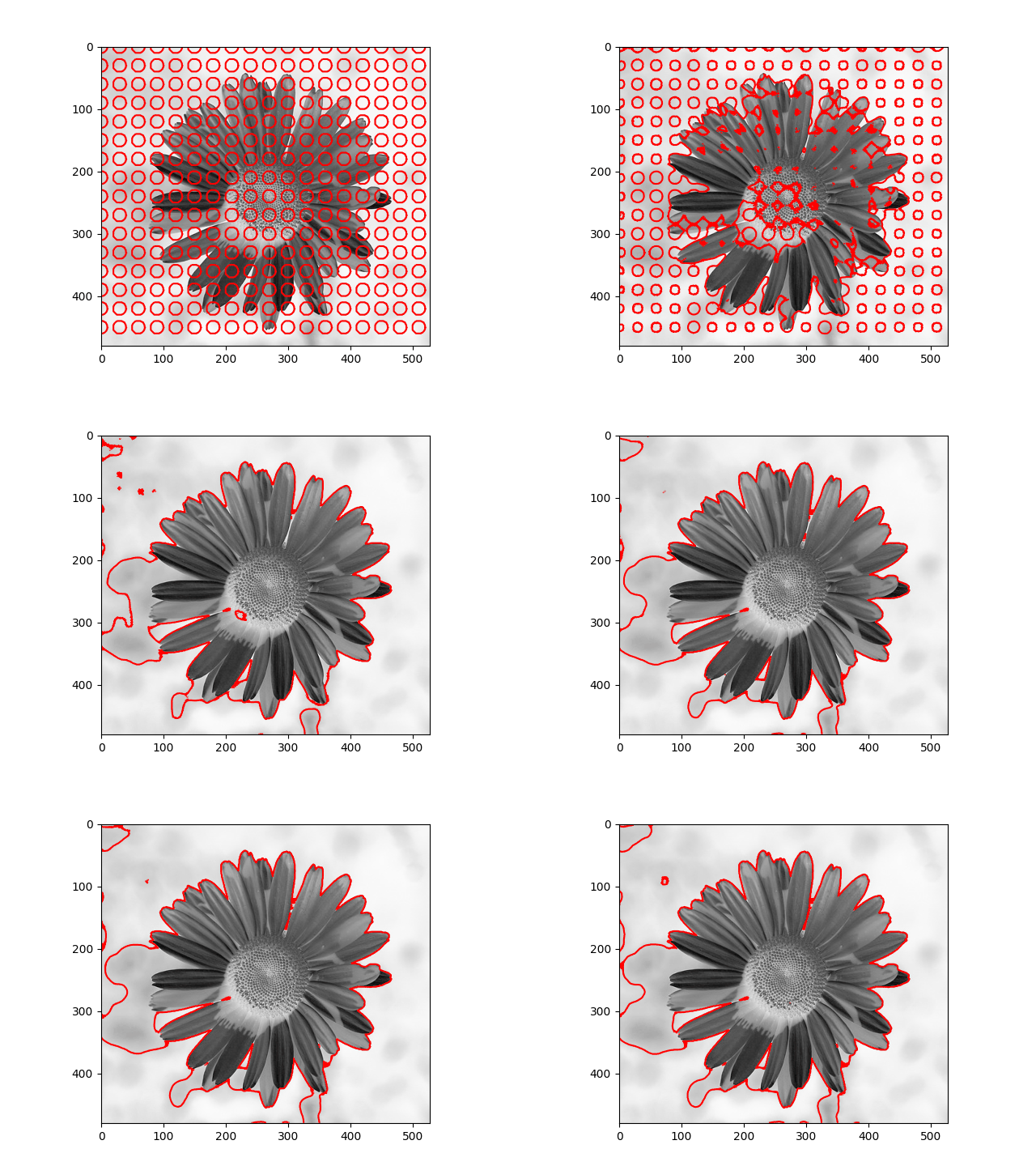
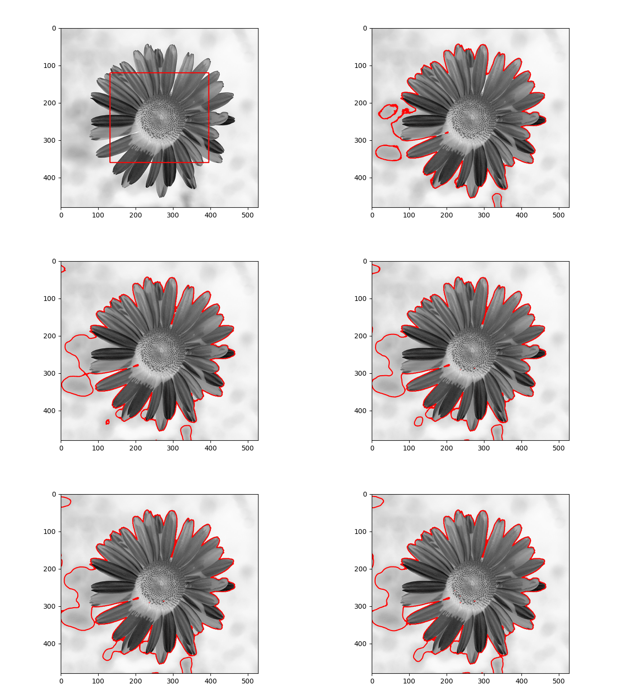
The distribution we used in the daisy samples is Single Variable Gaussian Distribution.
| Results | Results |
|---|---|
 |  |
Reference
[1] CREMERS, Daniel; ROUSSON, Mikael; DERICHE, Rachid. A review of statistical approaches to level set segmentation: integrating color, texture, motion and shape. International journal of computer vision, 2007, 72.2: 195-215.
