Variational Methods and Image Segmentation (Part 2)
Published:
After finishing Snakes problem in part 1, today, we will get into an improvement of it which is called Active Contours Without Edges. The reason it has “without edges” is that the model doesn’t use the image gradient information of the input image. You can also read the original version at here.
Formulation
Let $I: \Omega \rightarrow \mathbb{R}$ be a grayscale image, where $\Omega \subset \mathbb{R}^2$. The curve $C$ segments image $I$ into 2 partitions: $R_i$ - the region inside $C$, and $R_o$ - the region outside $C$.
Again, our goal is still to find $C$, which is equivalent to minimize energy function $E(C)$, but the energy function here is a little bit different to that one in part 1. Instead of using line integral, Chan Tony F et al. [1] used area integral over the image plane to evaluate the performance of segmentation:
\[E(C) = E_i(C) + E_o(C) = \iint_{R_i} |I(x,y) - c_i|^2 \, dx \, dy + \iint_{R_o} |I(x,y) - c_o|^2 \, dx \, dy\]where $c_i$ and $c_o$ respectively are the average $I(x,y)$ in $R_i$ and $R_o$.
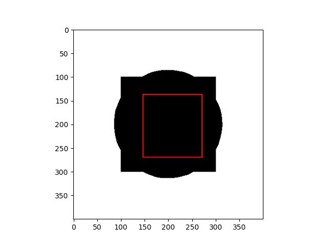
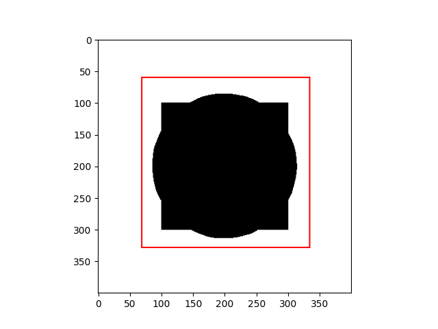
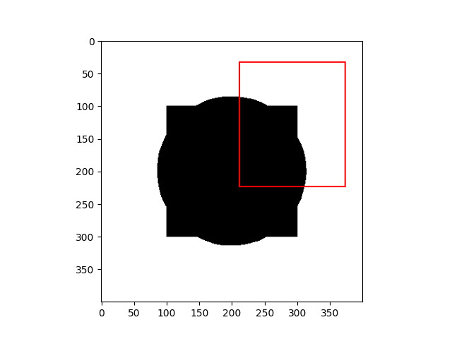
Intuitively, we can notice this energy function makes sense since:
- If the curve $C$ is inside an object, $E_i \approx 0$ and $E_o \gt 0$.
- If the curve $C$ is outside an object, $E_i \gt 0$ and $E_o \approx 0$.
- If the curve $C$ is both inside and outside an object, $E_i \gt 0$ and $E_o \gt 0$.
- If the curve $C$ can segment an object perfectly, $E_i \approx 0$ and $E_o \approx 0$.
| Curve inside an object | Curve outside an object |
|---|---|
 |  |
| Curve inside and outside an object | Curve fitting an object |
 |  |
Similar to the Snakes: Active Contours Model, TF Chan [1] would add some regularization terms into the energy function such as Length of curve $C$ and (or) Area of $R_i$. The terms guarantee the curve as small much as possible.
The energy function will be:
\[\begin{aligned} E(C, c_1, c_2) &= \mu \, \operatorname{Length}(C) + \nu \, \operatorname{Area}(\operatorname{inside}(C)) \\ &+ \lambda_1 \iint_{R_i} |I(x,y) - c_i|^2 \, dx \, dy \\ &+ \lambda_2 \iint_{R_o} |I(x,y) - c_o|^2 \, dx \, dy \end{aligned}\]The crucial step of this method is to replace an unknown curve $C: [0, 1] \rightarrow \Omega \subset \mathbb{R}^2$ by an unknown surface $\phi: \Omega \subset \mathbb{R}^2 \rightarrow \mathbb{R}$. The curve $C$, region inside $C$ - $R_i$ and outside $C$ - $R_o$ can be re-defined:
\[\begin{equation*} \begin{cases} C &= \{(x, y) \in \Omega \, | \, \phi(x, y) = 0\} \\ \operatorname{inside} (C) &= \{(x, y) \in \Omega \, | \, \phi(x, y) \gt 0\} \\ \operatorname{outside} (C) &= \{(x, y) \in \Omega \, | \, \phi(x, y) \lt 0\} \end{cases} \end{equation*}\]We can compute the length of curve $C$ and area of the region inside $C$ by using Heaviside step function ($H(.)$) and its derivative Dirac delta function ($\delta(.)$):
\[\begin{aligned} \operatorname{Length}(C) &= \iint_\Omega |\nabla H (\phi(x, y))| \, dx \,dy = \iint_\Omega \delta(\phi(x ,y))|\nabla \phi(x, y)| \, dx \,dy \\ \operatorname{Area}(R_i) &= \iint_\Omega H(\phi(x, y)) \, dx \, dy \end{aligned}\]where:
- Heaviside step function is defined: \(\begin{equation*} H(x) = \begin{cases} 1 & \quad x \ge 0, \\ 0 & \quad x \lt 0. \end{cases} \end{equation*}\)
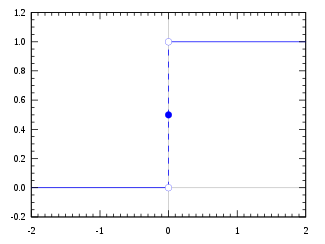
Heaviside step function
- Dirac delta function is defined: \(\begin{equation*} \delta(x) = \begin{cases} \infty & \quad x = 0 \\ 0 & \quad \text{otherwise} \end{cases} \end{equation*}\)
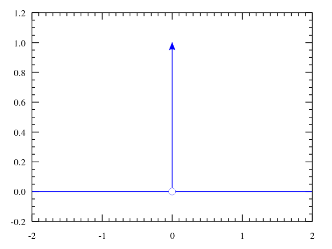
Dirac delta function
Finally, finding optimal curve $C$ is equivalent to find a level surface $\phi$ such that:
\[\begin{aligned} \phi, c_i, c_o = \underset{\phi, c_i, c_o}{\operatorname{arg\,min}} E(\phi, c_1, c_2) &= \iint_\Omega \mu \, \delta(\phi (x, y)) |\nabla \phi (x, y)| + \nu \, H(\phi (x, y))\\ &+ \lambda_1 H(\phi (x, y)) |I(x,y) - c_i|^2 + \lambda_2 (1 - H(\phi (x, y))) |I(x ,y) - c_o|^2 \, dx \, dy \end{aligned}\]Solution
Again, the method solving this problem is Euler - Lagrange Equation and gradient descent. We recommend you read the previous blog to familiarize yourself with the way we expand formulation.
\[\begin{aligned} E(\phi, c_i, c_o) &= \iint_\Omega \mu \, \delta(\phi (x, y)) |\nabla \phi (x, y)| + \nu \, H(\phi (x, y))\\ &+ \lambda_1 H(\phi (x, y)) |I(x,y) - c_i|^2 + \lambda_2 (1 - H(\phi (x, y))) |I(x ,y) - c_o|^2 \, dx \, dy \\ &= \iint_\Omega L(\phi, \nabla \phi, c_i, c_o) \, dx \, dy \end{aligned}\]The optimal $\phi$, $c_i$ and $c_o$ are:
\[\begin{aligned} \underset{\phi, c_i, c_o}{\operatorname{arg\,min}} \, E(\phi, c_1, c_2) = \iint_\Omega L(\phi, \nabla \phi, c_i, c_o) \, dx \, dy \end{aligned}\]To solve this, first, we would iteratively find optimal values/ function of each $c_i$, $c_o$, and $\phi$:
- Step 1: Considering $\phi$ and $c_o$ as constants, the optimal value of $c_i$ is: \(c_i = \dfrac{\iint_\Omega H(\phi (x, y)) I(x, y) \, dx \, dy}{\iint_\Omega I(x, y) \, dx \, dy}\)
Step 2: Considering $\phi$ and $c_i$ as constants, the optimal value of $c_o$ is: \(c_o = \dfrac{\iint_\Omega (1 - H(\phi (x, y))) I(x, y) \, dx \, dy}{\iint_\Omega I(x, y) \, dx \, dy}\)
- Step 3: Considering $c_i$ and $c_o$ as constants, update step of $\phi$ is: \(\dfrac{\partial \phi}{\partial t} = - \dfrac{dE}{d\phi} = \delta(\phi) \left( \mu \operatorname{div} \left(\dfrac{\nabla \phi}{|\nabla \phi|} \right) - \nu - \lambda_1 (I - c_i)^2 + \lambda_2 (I - c_o)^2 \right)\)
In the implementation, rather than having the Heaviside step and Dirac delta function as discrete functions, we replace them with their softer versions:
\[\begin{aligned} H(x) &= \dfrac{1}{2}\left( 1 + \dfrac{2}{\pi} \operatorname{arctan}\left( \dfrac{x}{\epsilon}\right)\right) \\ \delta(x) &= \dfrac{\epsilon^2}{\pi(\epsilon^2 + x^2)} \end{aligned}\]where $\epsilon = 10^{-6}.$
Results
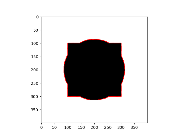
| Input Images | Results |
|---|---|
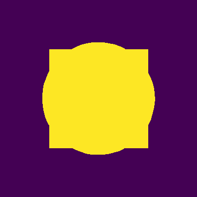 | 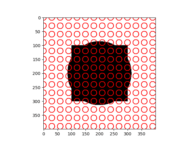 |
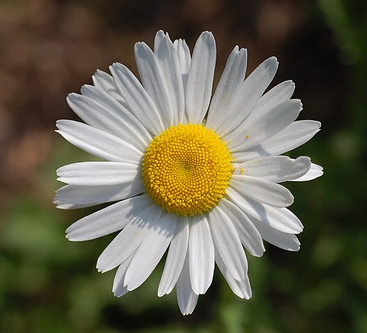 | 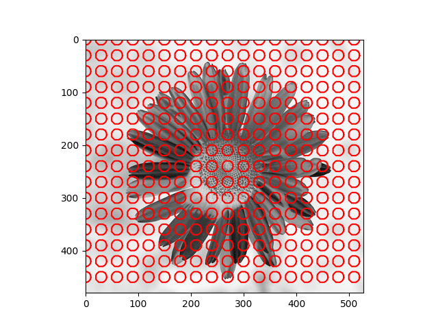 |
Discuss
The method depends heavily on the initial $\phi$ and the Euler - Lagrange equation, which is just a necessary condition - it doesn’t guarantee the global optimum, and sometimes the result maybe is the local optimum. As you can notice in the daisy flower sample, some regions in the background are recognized as the foreground, and the yellow disk flowers are the background.
Reference
[1] CHAN, Tony F.; VESE, Luminita A. Active contours without edges. IEEE Transactions on image processing, 2001, 10.2: 266-277.