
Variational Methods and Image Segmentation (Part 1)
Published:
Convolution neural networks usually appear in segmentation problems because of their high adaptation to many datasets and high performance. However, in return, they require ground truth data to learn and perform specific tasks, and without ground truth, their results are really poor. Today, I will introduce to you “old” segmentation methods, but they can be applied to several certain problems in the absence of datasets. This is called Snakes: Active Contours Models.
Formulation
Let $I: \Omega \rightarrow \mathbb{R}$ be a gray-scaled image, where $\Omega \subset \mathbb{R}^2$. The curve that segments image $I$ into 2 partitions is denoted as $C: [0, 1] \rightarrow \Omega$, in other words $C = (x(s), y(s))$ where $s \in [0, 1]$.
What we need to do is to find $C$.
But, there are innumerable curves $C$, so how do we know which one is the most suitable for a given image?
To answer that, we need some criteria for a good curve $C$:
- The input image’s two regions, foreground, and background, should be separated completely.
- The curve $C$ should be continuous and smooth as much as possible.
With the two above assumptions, we can derive an energy function to find $C$:
\[E(C) = E_\text{image}(C) + E_\text{int}(C)\]- For the first criterion, we can utilize the property of an image that is the drastic change of intensity in edge regions to detect foreground and background. The energy function $E_\text{image}(C)$ should force the curve toward that boundary of foreground and background region:
If the curve is at the flat region, the magnitude of the image gradient is zero, while when the curve is at the boundary, the magnitude is the largest. Because of this, the external energy is negative of image gradient magnitude. In addition, $E_\text{image}(C)$ is called external energy since it depends mainly on the input image.
The second criterion helps us derive an internal energy of curve $C$ which evaluates the continuity and smoothness of an arbitrary curve:
Continuity term:
\[E_\text{cont}(C) = \int_0^1 |C_s|^2 \, ds = \int_0^1 \left|\dfrac{\partial x}{\partial s}\right|^2 + \left|\dfrac{\partial y}{\partial s}\right|^2 ds\]Smoothness term:
\[E_\text{curve}(C) = \int_0^1 |C_{ss}|^2 \, ds = \int_0^1 \left|\dfrac{\partial^2 x}{\partial s^2}\right|^2 + \left|\dfrac{\partial^2 y}{\partial s^2}\right|^2 ds\]
The purpose of the energy is to penalize the non-continuous and non-smooth curve:
\[E_\text{int}(C) = \int_0^1 \alpha(s) |C_s|^2 + \beta(s) |C_{ss}|^2 \, ds\]Because of the diversity of objects needed to be segmented (some are really smooth, but others may be spiky), two weights $\alpha(s)$ and $\beta(s)$ are added to control the contribution of two small energy functions in the objective function.
Finally, finding the curve $C$ fulfilling these criteria is minimizing the total energy function (proposed by Kass et al [1]):
\[C = \underset{C}{\operatorname{arg min}} \, E(C) = \underset{C}{\operatorname{arg min}} \, \dfrac{1}{2} \int_0^1 - |\nabla I(C)|^2 + \alpha (s) |C_s|^2 + \beta (s) |C_{ss}| \, ds\]Solution
Euler - Lagrange equation
What we need to find right now is not a finite number of parameters but actually the function $C$ and how we minimize energy function $E$ where $C$ is an argument
According to Euler - Lagrange equation, the optimal function $f$ must hold the necessary condition (Read more here).
The energy function can be written in the form:
\[\begin{equation} E(C) = \int_0^1L(C, C_s, C_{ss}) \, ds \end{equation}\]And the necessary condition is:
\[\begin{equation} \dfrac{dE}{dC} = \dfrac{\partial L}{\partial C_s} - \dfrac{\partial}{\partial s}\left(\dfrac{\partial L}{\partial C_s}\right) + \dfrac{\partial ^ 2}{\partial s^2}\left(\dfrac{\partial L}{\partial C_{ss}}\right) = 0 \end{equation}\]In fact, this necessary condition does not guarantee that the solution is global optimum but only local optimum. However, at least we can still find an acceptable solution by using gradient descent.
Continue to expand the above equation and get the following:
Since $C = (x(s), y(s))$, we will take the derivative two times, with respect to $x$ and to $y$.
- $x = x(s)$
where $x^{(2)}$ and $x^{(4)}$ respectively, are the second and fourth order derivative of $x$ respect to $s$.
- $y = y(s)$
For the sake of simplicity, both weight parameters $\alpha(s)$ and $\beta(s)$ are considered as constants $\alpha$ and $\beta$.
Finite Difference
In reality, we define the curve $C$ by a set of points ${x_i, y_i}$ not by parametric functions, so to find $x^{(2)}$ and $x^{(4)}$, the central difference will be used. (Read more here)
\[\begin{aligned} x^{(2)}(s) &\approx \dfrac{x(s + h) - 2x(s) + x(s-h)}{h^2} \\ x^{(4)}(s) &\approx \dfrac{x(s + 2h) - 4x(s + h) + 6x(s) - 4x(s-h) + x(s - 2h)}{h^4} \\ \end{aligned}\]We can also rewrite these equations above in the matrix form.
\[\begin{equation} X^{(2)} \approx \left[\begin{array}{c} -2 & 1 & 0 & \cdots & 0 & 1 \\ 1 & -2 & 1 & \cdots & 0 & 0 \\ 0 & 1 & -2 & \cdots & 0 & 0 \\ \vdots & \vdots & \vdots & \ddots & \vdots & \vdots \\ 0 & 0 & 0 & \cdots & -2 & 1 \\ 1 & 0 & 0 & \cdots & 1 & -2\\ \end{array}\right] \left[\begin{array}{c} x_1 \\ x_2 \\ x_3 \\ \vdots \\ x_{n-1} \\ x_n \end{array}\right] = A_2 X \end{equation}\] \[\begin{equation} X^{(4)} \approx \left[\begin{array}{c} 6 & -4 & 1 & \cdots & 1 & -4 \\ -4 & 6 & -4 & \cdots & 0 & 1 \\ 1 & -4 & 6 & \cdots & 0 & 0 \\ \vdots & \vdots & \vdots & \ddots & \vdots & \vdots \\ 1 & 0 & 0 & \cdots & 6 & -4 \\ -4 & 1 & 0 & \cdots & -4 & 6\\ \end{array}\right] \left[\begin{array}{c} x_1 \\ x_2 \\ x_3 \\ \vdots \\ x_{n-1} \\ x_n \end{array}\right] = A_4 X \end{equation}\]Finally, the term $-\alpha x^{(2)} + \beta x^{(4)}$ in Euler - Lagrange equation above is rewritten as matrix form:
\[-\alpha A_2 X + \beta A_4X\]$Y^{(2)}$ and $Y^{(4)}$ go analogously.
Implicit Euler method
To simplify notation, let $A = -\alpha A_2 + \beta A_4$ and $P_x = I_xI_{xx} + I_yI_{yx}$.
The Euler - Lagrange equation becomes:
\[\dfrac{dE}{dX} = -P_x(X) + AX\]In this step, we will use the implicit Euler method and consider $P_x(X)$ as constant:
\[\dfrac{1}{\gamma}(X_t - X_{t+1}) = -P_x(X_t) + AX_{t+1}\]where $\gamma$ is the step size.
Finally, the $X_{t+1}$ is obtained by:
\[X_{t+1} = (\gamma A + I_d)^{-1}(\gamma P_x(X_t) + X_t)\]The update equation for $Y_{t+1}$ is the same:
\[Y_{t+1} = (\gamma A + I_d)^{-1}(\gamma P_y(Y_t) + Y_t)\]Results
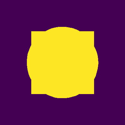
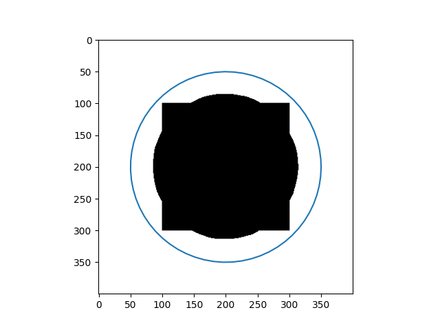
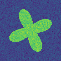
| Input Images | Results |
|---|---|
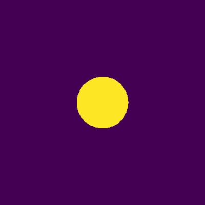 | 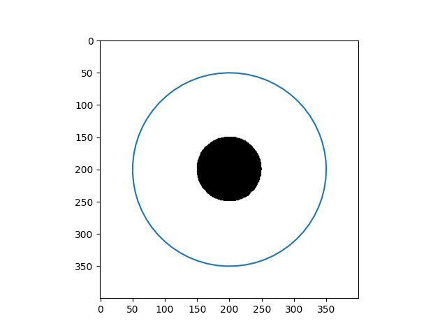 |
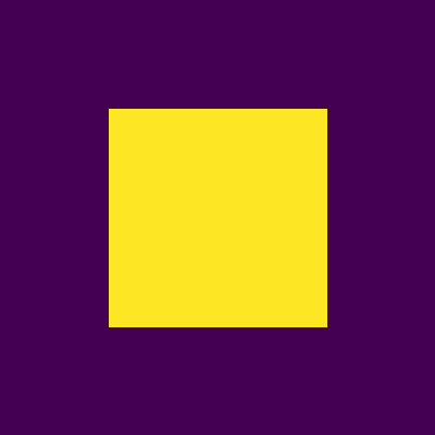 | 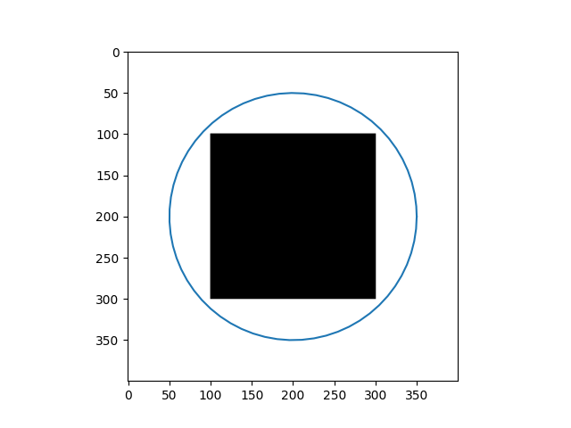 |
 |  |
 | 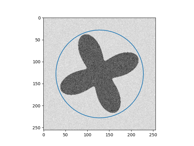 |
Discussion
One of the weaknesses of Snakes is its heavy reliance on the initialization of the curve $C$.
Failure Case
When the initial curve is inside the flattened foreground, it keeps shrinking to find the boundary and then vanishes.
This is due to the local search (doing line integral along the curve $C$). Many noticed this and replaced unknown curve $C$ with another unknown level surface $\Phi$. Read in part 2. :)
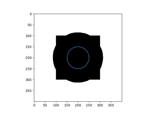
In addition, in implementation, two weighted parameters $\alpha(s)$ and $\beta(s)$ are treated as constants for the sake of simplicity during the optimization process. However, if we do not carefully choose values for the parameters, we cannot get the desired result, as you can see in the 4 - petal flower example, where the curve $C$ can not shrink to fit the boundary. Recently, Xu, Ziqiang, et al [2] fixed this by replacing $\alpha = \alpha(I)$ and $\beta = \beta(I)$ where $\alpha$ and $\beta$ are two encoder-decoder CNN, which is more flexible.
References
[1] Kass, Michael, Andrew Witkin, and Demetri Terzopoulos. “Snakes: Active contour models.” International journal of computer vision 1.4 (1988): 321-331.
[2] Xu, Ziqiang, et al. “CVNet: Contour Vibration Network for Building Extraction.” Proceedings of the IEEE/CVF Conference on Computer Vision and Pattern Recognition. 2022.