Variational Methods and Image Denoising
Published:
Variational methods are really powerful and have a variety of applications, such as 2D segmentation and 3D reconstruction. However, today I will present to you one of their interesting applications: Image Denoising.
Nowadays, the popularity and the adaptability power of CNNs are making engineers depend on more datasets with human-labeled ground truth, and the designing of CNNs like playing with Lego blocks, adding blocks, feeding a random input, and anticipating the desired output. But have you imagined how “our ancestors” can remove noise in an image without ground truth? If you do, let’s dive into mathematics :).
Formulation
Let $f: \Omega \rightarrow \mathbb{R}$ be a gray-scaled image on a domain $\Omega \in \mathbb{R}^2$. Assume that we observed a noisy image $u$ and want to recover to free-noise image $f$. However, we do not know noise sources (white noise or poison), additive noise, or multiplicate noise but only one noisy image $u$. To solve this inverse problem, we can have two assumptions based on our observation:
- The structure of $f$ should be similar as possible to that of $u$.
- $f$ should be spatially smooth.
With the two above assumptions, we can derive an energy function to find $f$:
\[\begin{align} E(f, u) &= E_\text{structure}(f, u) + E_\text{smoothness}(f) \\ \end{align}\]The similarity of two images $f$ and $u$ is computed by:
\[\begin{equation} E_\text{structure}(f, u) = \dfrac{1}{2}\iint_{\Omega} (f - u)^2 \text{d}x\,\text{d}y \end{equation}\]While the smoothness can be evaluated:
\[\begin{equation} E_\text{smoothness}(f) = \dfrac{1}{2}\iint_{\Omega} ||\nabla f||^2 \text{d}x \, \text{d}y \end{equation}\]where $\nabla f = <\partial f/\partial x, \partial f/ \partial y>$.
The optimal $f$ is:
\[\begin{aligned} \underset{f}{\operatorname{arg\,min}} \, E(f, u) &= \dfrac{1}{2}\iint_{\Omega} (f - u)^2 + \lambda ||\nabla f||^2 \, \text{d}x\,\text{d}y \\ &= \dfrac{1}{2}\iint_{\Omega} (f - u)^2 + \lambda (f_x^2 + f_y^2) \, \text{d}x\,\text{d}y \end{aligned}\]where $\lambda$ is a weighted number.
Solution
What we need to find right now is not a finite number of parameters but actually, the function $f$ and how we minimize energy function $E$ where $f$ is an argument.
According to Euler - Lagrange equation, the optimal function $f$ must hold the necessary condition (Read more here). The energy function can be written in the form:
\[\begin{equation} E(f, u) = \iint_{\Omega}L(f, f_x, f_y,u) \, \text{d}x \, \text{d}y \end{equation}\]And the necessary condition is:
\[\begin{equation} \dfrac{dE}{df} = \dfrac{\partial L}{\partial f} - \dfrac{\partial}{\partial x}\left(\dfrac{\partial L}{\partial f_x}\right) - \dfrac{\partial}{\partial y}\left(\dfrac{\partial L}{\partial f_y}\right) = 0 \end{equation}\]This necessary condition does not guarantee that the solution is global optimum but only local optimum. However, at least we can still find an acceptable solution by using gradient descent. (a small exercise for readers is to prove $E(f,u)$ strictly covex and with that strict convexity we can achieve global minima by gradient descent)
Continue to expand the above equation to get:
\[\begin{aligned} \dfrac{dE}{df} &= \dfrac{\partial L}{\partial f} - \dfrac{\partial}{\partial x}\left(\dfrac{\partial L}{\partial f_x}\right) - \dfrac{\partial}{\partial y}\left(\dfrac{\partial L}{\partial f_y}\right) \\ &= (f - u) - \lambda \dfrac{\partial}{\partial x}f_x - \lambda \dfrac{\partial}{\partial y}f_y \\ &= (f - u) - \lambda(f_{xx} + f_{yy}) \end{aligned}\]Algorithm
The main algorithm is:
Step 1: Initialize the first function $f_0$
Step 2: Update $f_{t+1}$
Step 3:
If $E(f_{t + 1}, u) < \epsilon$, stop the algorithm,
else repeat step 2
Code
def denoise(noisy_image, n_iters):
    noisy_image = np.copy(noisy_image).astype(np.float32)
    denoised_image = np.copy(noisy_image)
    weight = 1
    step = 0.5

    for _ in range(n_iters):
        grad_y, grad_x = np.gradient(denoised_image)

        _, grad_xx = np.gradient(grad_x)
        grad_yy, _ = np.gradient(grad_y)

        grad = (noisy_image - denoised_image) + weight * (grad_xx + grad_yy)
        denoised_image = np.clip(denoised_image + step * grad, 0, 255)

    return denoised_image
Result
| Noisy Image | Denoised Image |
|---|---|
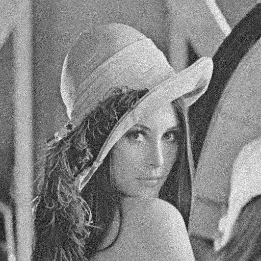 | 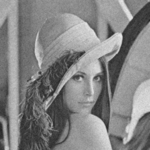 |
Discussion
Alternative for Smoothness Term
Regarding the energy function above, since the $E_\text{structure}$ is fixed in order to preserve the image structure while optimizing, people usually tweak and modify $E_\text{smoothness}$ to achieve desired results. Total variation $L_1$ term can be an alternative for $L_2$ which makes edges in an image sharper instead of blurrier:
\[E_\text{smoothness}(f) = \int_\Omega ||\nabla f|| \, \text{d}x \, \text{d}y = \int_\Omega \sqrt{f_x^2 + f_y^2} \, \text{d}x \, \text{d}y\]and the update equation for image function $f$ is:
\[\begin{aligned} \dfrac{df}{dt} = -\dfrac{dE}{df} &= -\dfrac{\partial L}{\partial f} + \dfrac{\partial}{\partial x}\left(\dfrac{\partial L}{\partial f_x}\right) + \dfrac{\partial}{\partial y}\left(\dfrac{\partial L}{\partial f_y}\right) \\ &= (u - f) + \lambda \dfrac{\partial}{\partial x}\left(\dfrac{f_x}{\sqrt{f_x^2 + f_y^2}}\right) + \lambda \dfrac{\partial}{\partial y}\left(\dfrac{f_y}{\sqrt{f_x^2 + f_y^2}}\right) \\ &= (u - f) + \lambda \operatorname{div}\left(\dfrac{\nabla f}{||\nabla f||}\right) \end{aligned}\]| Noisy Image | $L_2$ Denoised Image | $L_1$ Denoised Image |
|---|---|---|
| | 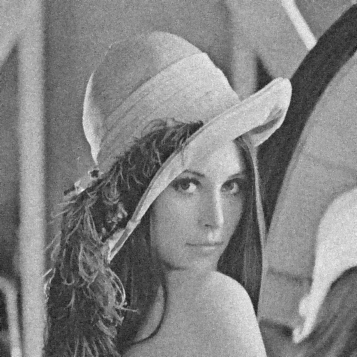 |
We can easily notice that the image used $L_1$ loss is shaper than the one used $L_2$.
The smoothness term $L_1$ and its variations are usually used beside the difference between predicted images and ground truths while training CNN-based image denoising models to preserve the clarity of detail in photos.
Contrast to Deep Learning
The formulation of DL image denoising methods is a little bit different from variational methods, which is:
\[\theta = \underset{\theta}{\operatorname{arg min}} \, ||g_\theta(\textbf{y}) - \textbf{x}||_p\]where $\textbf{y}$ is observed noisy image, $\textbf{x}$ is clean image and $g_\theta(.)$ is a CNN-based denoising model with parameters $\theta$.
However, having a realistic ground truth image may be a challenging problem in this field since shot noise (photon noise) is inevitable when capturing a realistic image (ground truth is achieved by averaging a burst image - a set of images captured within a small period of time). The image quality of result images of CNN-based methods usually is better than traditional, but normally only works on trained datasets. In some works like medical image denoising, where ground truths are impossible to achieve, self-supervised methods like variational methods or recently noise2noise[2], noise2void[3] are preferred.
Reference
[1] Rudin, L. I.; Osher, S.; Fatemi, E. (1992). “Nonlinear total variation based noise removal algorithms”. Physica D. 60 (1–4): 259–268
[2] Lehtinen, Jaakko, et al. “Noise2Noise: Learning image restoration without clean data.” arXiv preprint arXiv:1803.04189 (2018).
[3] Krull, Alexander, Tim-Oliver Buchholz, and Florian Jug. “Noise2void-learning denoising from single noisy images.” Proceedings of the IEEE/CVF conference on computer vision and pattern recognition. 2019.