Video Stabilization
Published:
Video stabilization is a process that aims to reduce the vibration and jitter inside videos.
Formulation
In video visualization, the input and output of the problem are obvious:
- Input: Initial image sequence ${I_i}$.
- Output: Stabilized image sequence ${I’_i}$.
where $I_i, I’_i: \Omega: \rightarrow \mathbb{R}^3$ are RGB image in domain $\Omega \subset \mathbb{R}^2$.
As we mentioned before, the movement of a camera recording a video is not perfect, which leads to vibration inside videos. Our goal is to smooth that movement to get stable frames.
![]()
Figure 1: Correlation between the unstable frame and the stable
Due to the imperfection of the real camera’s pose (“noise - vibration” in the camera’s pose), we need to find a virtual camera, that is more stable than the original. The difference between these two cameras can be presented by a transformation matrix $G$.
Expanding this to all shaky frames, we have this:
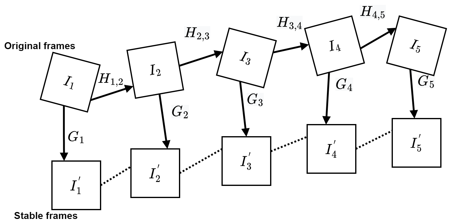
where the transformation matrix $H_{i, i+1}$ presents the movement of the camera from frame $I_i$ to frame $I_{i + 1}$ and $G_i$ is the stabilizing transformation matrix.
Our goal now is clearer - finding ${G_i}$.
Framework
Traditional video stabilization methods all use the same framework, which is:
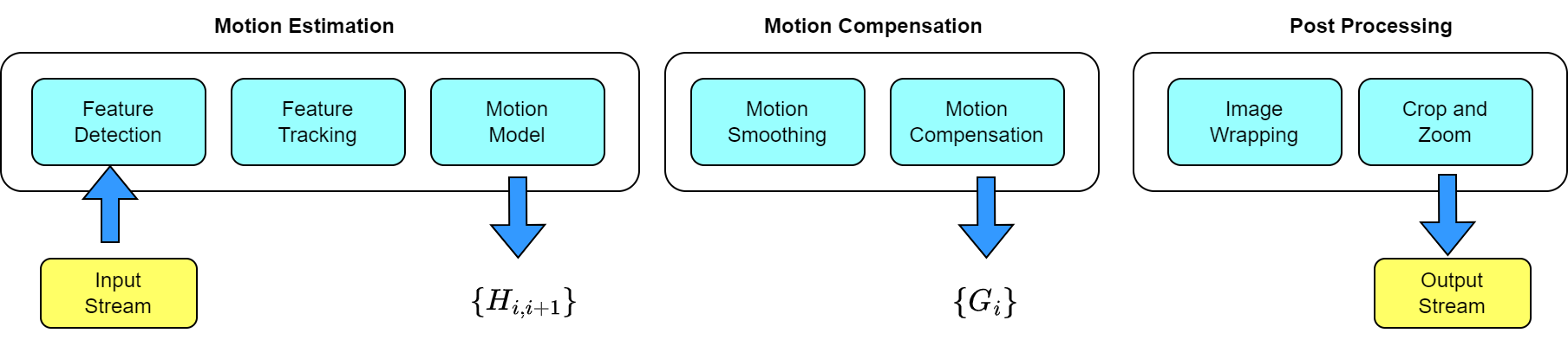
The framework includes three main steps:
- Motion estimation: used to estimate the camera movement
- Motion compensation: smoothing the camera motion and estimating transformation matrix G for each frame
- Post Processing: applying the transformation to each frame and reducing side effects
Motion Estimation
Feature Detection and Tracking
To stabilize frames, we must know the camera movement, but we do not have any information on camera movement in the world space. One way of estimating the camera movement is based on the motion vectors of features inside the image. So, we need to find image features and track them over time.
These algorithms are usually used:
- SHIFT/ SURF
- ORB/ FAST
- Harris Corners + KLT tracker.
Motion Model
After detecting and tracking features, we have pairs of corresponding key points \(\{(p^i_{k}, p^{i+1}_{k})\}\) of two successive frames $I_i$ and $I_{i+1}$.
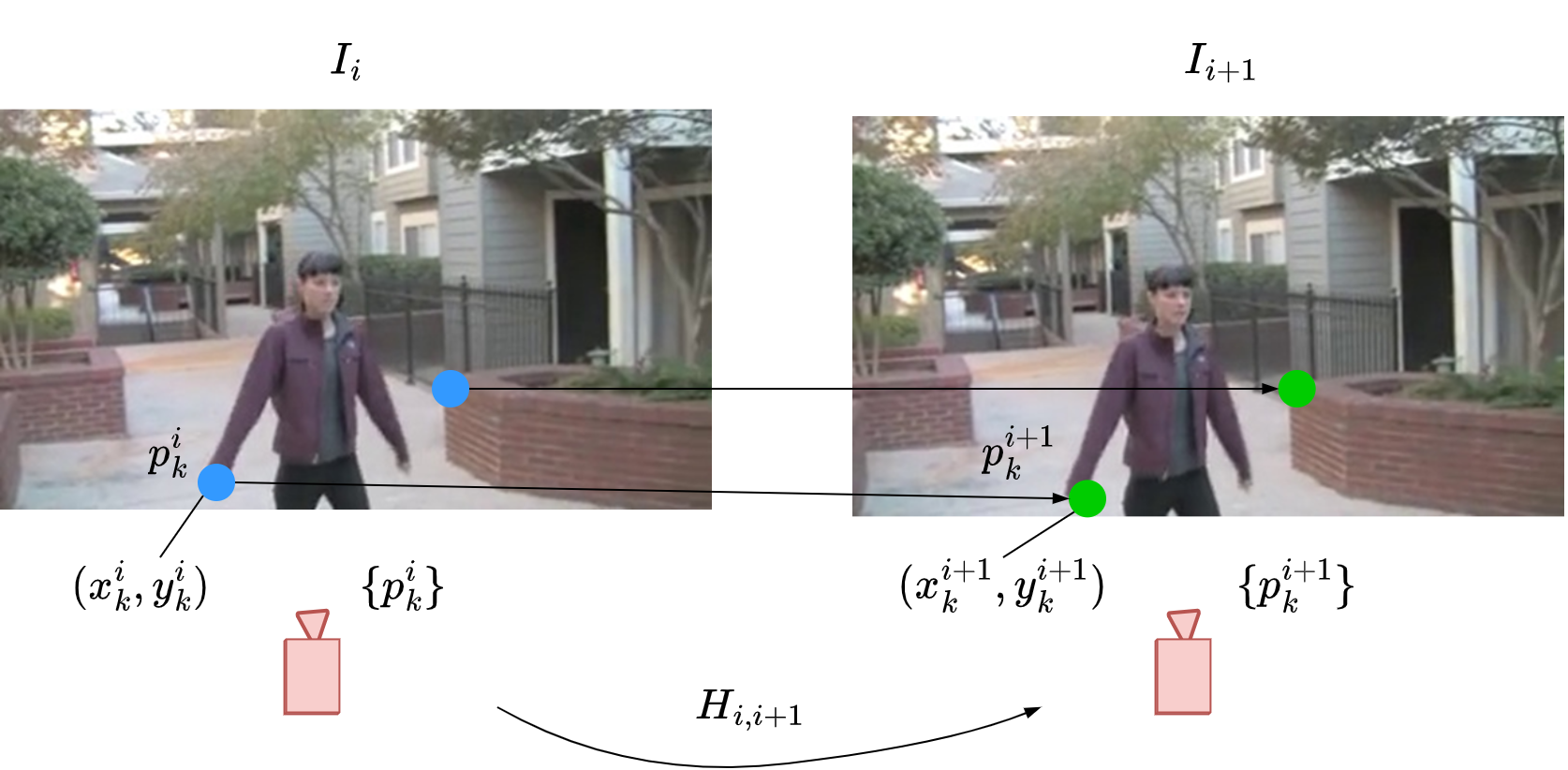
With the assumption that the transformation matrix $H_{i, i+1}$ between two frames is a homography with eight unknown parameters, we have the formulation:
\[\begin{aligned} w' \textbf{p}^{i+1}_k &= H_{i, i+1} \textbf{p}^i_k \\ w'\left[\begin{matrix} x_k^{i + 1} \\ y_k^{i + 1} \\ 1 \end{matrix}\right] &= \left[ \begin{matrix} h_{11} & h_{12} & h_{13} \\ h_{21} & h_{22} & h_{23} \\ h_{31} & h_{32} & 1 \end{matrix} \right] \left[ \begin{matrix} x_k^{i} \\ y_k^{i} \\ 1 \end{matrix}\right] \end{aligned}\]where $\textbf{p}$ is homogeneuos form of $p$.
With $n$ pairs of corresponding key points ${(p^i_k, p^{i+1}_k)}$, we will have $n$ similar homography equations as above.
To find these eight parameters, we will rewrite the homography equation to the linear system: \(A \cdot h = b\) where $h^T =[h_{11}, h_{12}, h_{13}, h_{21}, h_{22},h_{23}, h_{31}, h_{32}, 1]$ is unknown vector with 8 parameters.
So, we need at least eight equations to solve, but more equations are better since there may be errors/ noise in previous steps.
The linear system above can be solved by the Jacobi method, close form or least square, etc.
In addition, it depends on our assumption of camera movement between two successive frames. If we suppose that the camera translates, the number of parameters needed to find is just 2. But, the more parameters, the more accurate camera movement we can find.
![]()
Motion Compensation
Motion Smoothing
First, we have an assumption that the first original frame $I_1$ is always stable.
![]()
Because of the linearity of transformation matrices, we can find the cumulative transformation matrix $H_{1,i}$ transforming original frame $I_1$ to original frame $I_i$ by:
\[H_{1,i} = \prod_{k=2}^{i}H_{k-1,k} = H_{i-1, i}...H_{2,3}H_{1,2}\]Due to vibration while camera is moving, sequence ${H_{1,i}}$ will have noise, which lead to frames ${I_i}$ unstable. What we have to do is to smooth ${H_{1, i}}$.
Suppose that smoothed matrix \(\bar{H}_{1, i}\) of \(H_{1, n}\) with gaussian convolution:
\[\bar{H}_{1, i} = \operatorname{smooth}(..., H_{1, i - 1}, H_{1, i}, H_{1, i + 1}, ...)\]is the transformation matrix from the first stable frame $I_1$ to the stable frame $I_i’$.
with $\operatorname{smooth}(.)$ being an element wise gaussian convolution operator.
Motion Compensation
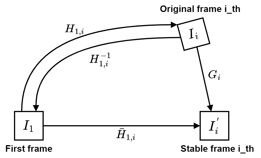
After estimating $\bar{H}_{1,i}$, we can easily find the stabilizing matrix $G_i$ by:
\[G_i = \bar{H}_{1,i} \cdot H^{-1}_{1,i}\]Post-processing
To get a stabilize frame $I_i’$, we just wrap $I_i$ with $G_i$ by applying the equation:
\[I_i'(G_i \textbf{x}) = I_i(\textbf{x})\]with $\textbf{x} = [x, y, 1]^T$.
After stabilizing frame $I_i$, we also need to eliminate empty space in the transformed image. This step is called “crop and zoom.”
Results
This is an example after being applied the above strategy. The scene is static ( there is not any moving object inside the video).
| Shaky Video | Stabilized but Uncropped Video | Fully Processed Video |
|---|---|---|
 |  |  |
This video was recorded by a man while he was walking on the street. There are some moving people in the video but not too many, and their sizes are small. Some details, like trees, are distorted after being stabilized.
| Shaky Video | Stabilized but Uncropped Video | Fully Processed Video |
|---|---|---|
 |  |  |
This video recorded a dancing woman, and also, there are some jitters inside it. The output is really bad. Because our assumption only deals with a static scene. In this example, it is no longer true.
| Shaky Video | Stabilized but Uncropped Video |
|---|---|
|  |
You can read [1] to know more about other assumptions as well as different smoothing strategies.
Reference
[1] Sánchez, Javier. “Comparison of motion smoothing strategies for video stabilization using parametric models.” Image Processing On Line (2017).