
Harris Corner Detection
Published:
A Corner is a point whose local neighborhood stands in two dominant and different edge directions. In other words, a corner can be interpreted as the junction of two edges, where an edge is a sudden change in image brightness. Corners are the important features in the image, and they are generally termed as interest points that are invariant to translation, rotation, and illumination.
Formulation and Solution
The Harris corner detector uses the geometry property of corners to detect them. As you see in the first image in figure 2, the content of the green window does not change when we shift the window in all directions. In the second, when the window lies on edges, its content does not change along the edge direction, only changes when shifting in other directions. Finally, in cases the window lies on a corner, the content of the window varies when we shift it in all directions. So, we will find the corner region by placing a window in that place, if window content varies strongly in all directions, that region is the corner. The window content varies strongly definition is measured by taking sum of square distance (SSD).
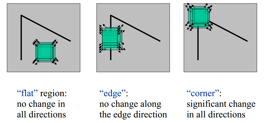
Figure 2: Intuition of Harris Corner Detector
The variation can be defined as a sum of square distance (SSD) as below, $(u, v)$ denotes the shift vector, $W$ is the region needed to determine, $w(x,y)$ is a window function, $I(x,y)$ is image function, and at coordinate $(x, y)$, the image has a certain intensity. The window function usually chosen is a rectangle or gaussian function.
\[E(u, v) \approx \sum_{(x, y) \, \in \,W} w(x, y) \, [\,I(x + u, y+ v) - I(x, y)\,] \,^ {2}\]The energy function value of $E(u, v)$ in the region $W$ should be large for any shift.
The shifted intensity can be approximated by Taylor expansion:
\[I (x + u, y + v) \approx I(x, y) + u\,I_{x} (x,y) + v\,I_{y} (x,y) + R_{2}\]Therefore, the SSD measure is now:
\[\begin{aligned} E(u, v) & \approx \sum_{(x, y)\, \in \,W} w(x, y)\,[\,u\,I_{x} (x,y) + v\,I_{y} (x,y)\,]\,^{2} \\ & = \sum_{(x, y)\, \in \,W} w(x, y)\, [u \quad v] \left[\begin{array}{cc} I_{x}^{\,2}&I_{x}\,I_{y}\\ I_{x}\,I_{y}&I_{y}^{\,2} \end{array}\right] \left[\begin{array}{c} u\\v \end{array}\right]\\ & = [u \quad v] \Biggl ( \sum_{(x, y)\, \in \,W} w(x, y)\, \left[\begin{array}{cc} I_{x}^{\,2}&I_{x}\,I_{y}\\ I_{x}\,I_{y}&I_{y}^{\,2} \end{array}\right] \Biggr) \left[\begin{array}{c} u\\v \end{array}\right]\\ & = \mathbf{u^{T}} \, M \, \mathbf{u}. \end{aligned}\]Because $M$ is a real and symmetric matrix, it can be decomposed to be:
\[M = Q \, \Lambda \, Q^{T}.\]where $Q$ is orthogonal matrix and $\Lambda$ is diagonal matrix. So the SSD measure can be written again:
\[\begin{aligned} E(\mathbf{u}) & = \mathbf{u^{T}} \, M \, \mathbf{u} = \mathbf{u^{T}} \, Q \, \Lambda \, Q^{T} \, \mathbf{u} = (Q^{\mathbf{T}} \, \mathbf{u})^{\mathbf{T} } \, \Lambda \, (Q^{\mathbf{T}} \, \mathbf{u}) \\ & = \mathbf{u'^{T}} \, \Lambda \, \mathbf{u'} = \lambda_1 \, ||\mathbf{u'}||_2^{2} + \lambda_2 \, ||\mathbf{u'}||_2^{2}. \end{aligned}\]where $\lambda_1$ and $\lambda_2$ is eigen values of $M$. We want $E(\mathbf{u})$ to be big for all directions $\mathbf{u}$ so both $\lambda_1$ and $\lambda_2$ must be large. If both are small, it will be “flat”. For “edge” case, one large eigen value and one small eigen value.
The Harris detector specially is designed a response:
\[\begin{aligned} R & = det(M) - k \, trace(M)^{2} \\ & = \lambda_1 \lambda_2 - k \, (\lambda_1 +\lambda_2)^{2}. \end{aligned}\]The parameter k is usually set to between 0.04 and 0.06. If $R$ is large, it is a corner. Otherwise negative $R$, it’ll be edge; positive $R$ but small, the flat region.
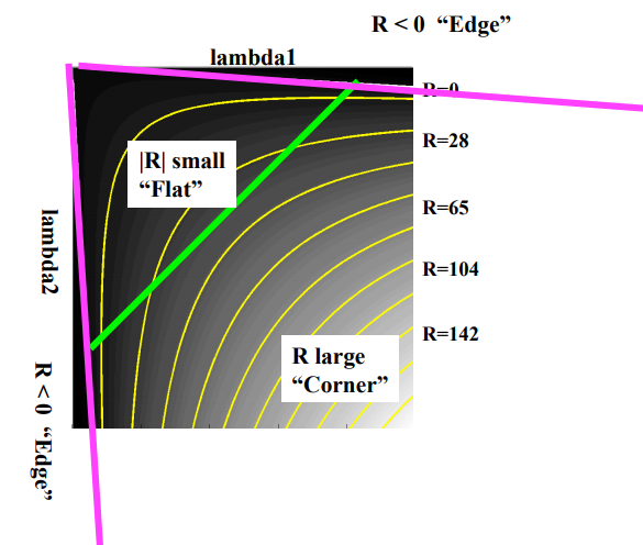
Figure 3: Harris Region
In addition, Shi-Tomasi proposed the scoring function as:
\(R = min (\lambda_ 1, \lambda_2)\) which basically means if $R$ is greater than a threshold, it is classified as a corner.
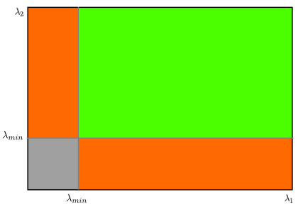
Figure 4: Shi-Tomashi Region
Finally, the method is applied non - max suppression algorithm to remove redundant points.