Optical Flow

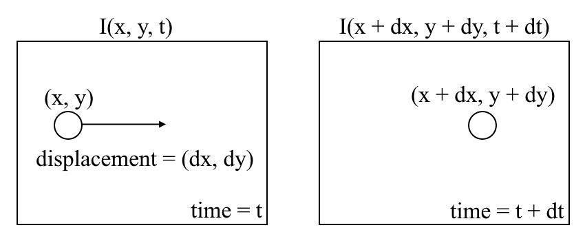
Optical flow is the pattern of appearance of objects’ motion in an image, between two successive frames caused by the movement of objects or the camera. It is a 2D vector field, where each vector represents a displacement or movement of features from a first frame to a second frame (see the below image).

Assumption and Formulation

The problem:

Being given 2 successive frames $I_1$ and $I_2$, we need to find the motion vector $(dx, dy)$ for each pixel.

To solve this problem, Horn & Schunck had made some assumptions:

1. Images are captured in ambient light: This means that the intensity of pixels does not depend on the position of the camera.

2. Spatial Motion: Pixels do not move fast.

3. Spatial Correlation: All neighbors of one pixel also have the same motion as the center one.

After having some assumptions, the problem can be solved easily.

The first assumption let we have the equation: $I(x, y, t) = I(x + dx, y + dy, t + dt)$

The second assumption means that $dx$, $dy$, $dt$ are very small, so that we can approximate $I(x + dx, y + dy, t + dt)$ with the first order of Taylor series:

$I(x + dx, y + dy, t + dt) \approx I(x, y, t) + \nabla I_x dx + \nabla I_y dy + \nabla I_t dt.$

Because we are considering 2 successive frames ($dt = 1$), we have:

$I(x, y, t) = I(x + dx, y + dy, t + dt) \approx I(x, y, t) + \nabla I_x dx + \nabla I_y dy + \nabla I_t.$

$\rightarrow \nabla I_x dx + \nabla I_y dy + \nabla I_t \approx 0.$ (1)

Where $\nabla I_x$, $\nabla I_y$, $\nabla I_t$ are derivatives of image $I$ with respect to x - axis, y-axis, and time.

$\nabla I_x (x, y)= I_t (x + 1, y) - I_t (x - 1, y)$.

$\nabla I_y (x, y)= I_t (x, y + 1) - I_t (x, y - 1)$.

$\nabla I_t (x, y)= I_{t + 1} (x, y) - I_t(x, y)$.

To find $dx$, $dy$ in equation (1), we need at least 2 equations, and the last assumption will help us.

In the third assumption, all neighbors of a pixel will have the same motion. So, we can assume that a $3\times3$ region around a pixel will have the same motion. Now we have 9 equations, so we can solve equation (1).

The equation above can be considered as a linear system: $Ax = b$ with $x^T = \left[dx \quad dy\right]$.

There are a lot of methods used to solve this equation: Close form, Pseudo Inverse, Least squares, Gaussian elimination, Jacobi method, and Gauss–Seidel method. Or even, you can utilize SVD to solve.